Aggregating and Analyzing Data with dplyr
Overview
Teaching: 40 min
Exercises: 15 minQuestions
How can I manipulate data frames without repeating myself?
Objectives
Describe what the
dplyrpackage in R is used for.Apply common
dplyrfunctions to manipulate data in R.Employ the ‘pipe’ operator to link together a sequence of functions.
Employ the ‘mutate’ function to apply other chosen functions to existing columns and create new columns of data.
Employ the ‘split-apply-combine’ concept to split the data into groups, apply analysis to each group, and combine the results.
Bracket subsetting is handy, but it can be cumbersome and difficult to read, especially for complicated operations.
Luckily, the dplyr
package provides a number of very useful functions for manipulating data frames
in a way that will reduce repetition, reduce the probability of making
errors, and probably even save you some typing. As an added bonus, you might
even find the dplyr grammar easier to read.
Here we’re going to cover 6 of the most commonly used functions as well as using
pipes (%>%) to combine them.
glimpse()select()filter()group_by()summarize()mutate()
Packages in R are sets of additional functions that let you do more
stuff in R. The functions we’ve been using, like str(), come built into R;
packages give you access to more functions. You need to install a package and
then load it to be able to use it.
install.packages("dplyr") ## install
You might get asked to choose a CRAN mirror – this is asking you to choose a site to download the package from. The choice doesn’t matter too much; I’d recommend choosing the RStudio mirror.
library("dplyr") ## load
You only need to install a package once per computer, but you need to load it every time you open a new R session and want to use that package.
What is dplyr?
The package dplyr is a fairly new (2014) package that tries to provide easy
tools for the most common data manipulation tasks. This package is also included in the tidyverse package, which is a collection of eight different packages (dplyr, ggplot2, tibble, tidyr, readr, purrr, stringr, and forcats). It is built to work directly
with data frames. The thinking behind it was largely inspired by the package
plyr which has been in use for some time but suffered from being slow in some
cases. dplyr addresses this by porting much of the computation to C++. An
additional feature is the ability to work with data stored directly in an
external database. The benefits of doing this are that the data can be managed
natively in a relational database, queries can be conducted on that database,
and only the results of the query returned.
This addresses a common problem with R in that all operations are conducted in memory and thus the amount of data you can work with is limited by available memory. The database connections essentially remove that limitation in that you can have a database that is over 100s of GB, conduct queries on it directly and pull back just what you need for analysis in R.
Taking a quick look at data frames
Similar to str(), which comes built into R, glimpse() is a dplyr function that (as the name suggests) gives a glimpse of the data frame.
Rows: 801
Columns: 29
$ sample_id     <chr> "SRR2584863", "SRR2584863", "SRR2584863", "SRR2584863", …
$ CHROM         <chr> "CP000819.1", "CP000819.1", "CP000819.1", "CP000819.1", …
$ POS           <dbl> 9972, 263235, 281923, 433359, 473901, 648692, 1331794, 1…
$ ID            <lgl> NA, NA, NA, NA, NA, NA, NA, NA, NA, NA, NA, NA, NA, NA, …
$ REF           <chr> "T", "G", "G", "CTTTTTTT", "CCGC", "C", "C", "G", "ACAGC…
$ ALT           <chr> "G", "T", "T", "CTTTTTTTT", "CCGCGC", "T", "A", "A", "AC…
$ QUAL          <dbl> 91.0000, 85.0000, 217.0000, 64.0000, 228.0000, 210.0000,…
$ FILTER        <lgl> NA, NA, NA, NA, NA, NA, NA, NA, NA, NA, NA, NA, NA, NA, …
$ INDEL         <lgl> FALSE, FALSE, FALSE, TRUE, TRUE, FALSE, FALSE, FALSE, TR…
$ IDV           <dbl> NA, NA, NA, 12, 9, NA, NA, NA, 2, 7, NA, NA, NA, NA, NA,…
$ IMF           <dbl> NA, NA, NA, 1.000000, 0.900000, NA, NA, NA, 0.666667, 1.…
$ DP            <dbl> 4, 6, 10, 12, 10, 10, 8, 11, 3, 7, 9, 20, 12, 19, 15, 10…
$ VDB           <dbl> 0.0257451, 0.0961330, 0.7740830, 0.4777040, 0.6595050, 0…
$ RPB           <dbl> NA, 1.000000, NA, NA, NA, NA, NA, NA, NA, NA, 0.900802, …
$ MQB           <dbl> NA, 1.0000000, NA, NA, NA, NA, NA, NA, NA, NA, 0.1501340…
$ BQB           <dbl> NA, 1.000000, NA, NA, NA, NA, NA, NA, NA, NA, 0.750668, …
$ MQSB          <dbl> NA, NA, 0.974597, 1.000000, 0.916482, 0.916482, 0.900802…
$ SGB           <dbl> -0.556411, -0.590765, -0.662043, -0.676189, -0.662043, -…
$ MQ0F          <dbl> 0.000000, 0.166667, 0.000000, 0.000000, 0.000000, 0.0000…
$ ICB           <lgl> NA, NA, NA, NA, NA, NA, NA, NA, NA, NA, NA, NA, NA, NA, …
$ HOB           <lgl> NA, NA, NA, NA, NA, NA, NA, NA, NA, NA, NA, NA, NA, NA, …
$ AC            <dbl> 1, 1, 1, 1, 1, 1, 1, 1, 1, 1, 1, 1, 1, 1, 1, 1, 1, 1, 1,…
$ AN            <dbl> 1, 1, 1, 1, 1, 1, 1, 1, 1, 1, 1, 1, 1, 1, 1, 1, 1, 1, 1,…
$ DP4           <chr> "0,0,0,4", "0,1,0,5", "0,0,4,5", "0,1,3,8", "1,0,2,7", "…
$ MQ            <dbl> 60, 33, 60, 60, 60, 60, 60, 60, 60, 60, 25, 60, 10, 60, …
$ Indiv         <chr> "/home/dcuser/dc_workshop/results/bam/SRR2584863.aligned…
$ gt_PL         <dbl> 1210, 1120, 2470, 910, 2550, 2400, 2080, 2550, 11128, 19…
$ gt_GT         <dbl> 1, 1, 1, 1, 1, 1, 1, 1, 1, 1, 1, 1, 1, 1, 1, 1, 1, 1, 1,…
$ gt_GT_alleles <chr> "G", "T", "T", "CTTTTTTTT", "CCGCGC", "T", "A", "A", "AC…
In the above output, we can already gather some information about variants, such as the number of rows and columns, column names, type of vector in the columns, and the first few entries of each column. Although what we see is similar to outputs of str(), this method gives a cleaner visual output.
Selecting columns and filtering rows
To select columns of a data frame, use select(). The first argument to this function is the data frame (variants), and the subsequent arguments are the columns to keep.
select(variants, sample_id, REF, ALT, DP)
# A tibble: 6 x 4
  sample_id  REF      ALT          DP
  <chr>      <chr>    <chr>     <dbl>
1 SRR2584863 T        G             4
2 SRR2584863 G        T             6
3 SRR2584863 G        T            10
4 SRR2584863 CTTTTTTT CTTTTTTTT    12
5 SRR2584863 CCGC     CCGCGC       10
6 SRR2584863 C        T            10
To select all columns except certain ones, put a “-“ in front of the variable to exclude it.
select(variants, -CHROM)
# A tibble: 6 x 28
  sample_id    POS ID    REF   ALT    QUAL FILTER INDEL   IDV   IMF    DP    VDB
  <chr>      <dbl> <lgl> <chr> <chr> <dbl> <lgl>  <lgl> <dbl> <dbl> <dbl>  <dbl>
1 SRR25848…   9972 NA    T     G        91 NA     FALSE    NA  NA       4 0.0257
2 SRR25848… 263235 NA    G     T        85 NA     FALSE    NA  NA       6 0.0961
3 SRR25848… 281923 NA    G     T       217 NA     FALSE    NA  NA      10 0.774
4 SRR25848… 433359 NA    CTTT… CTTT…    64 NA     TRUE     12   1      12 0.478
5 SRR25848… 473901 NA    CCGC  CCGC…   228 NA     TRUE      9   0.9    10 0.660
6 SRR25848… 648692 NA    C     T       210 NA     FALSE    NA  NA      10 0.268
# … with 16 more variables: RPB <dbl>, MQB <dbl>, BQB <dbl>, MQSB <dbl>,
#   SGB <dbl>, MQ0F <dbl>, ICB <lgl>, HOB <lgl>, AC <dbl>, AN <dbl>, DP4 <chr>,
#   MQ <dbl>, Indiv <chr>, gt_PL <dbl>, gt_GT <dbl>, gt_GT_alleles <chr>
To choose rows, use filter():
filter(variants, sample_id == "SRR2584863")
# A tibble: 6 x 29
  sample_id  CHROM    POS ID    REF   ALT    QUAL FILTER INDEL   IDV   IMF    DP
  <chr>      <chr>  <dbl> <lgl> <chr> <chr> <dbl> <lgl>  <lgl> <dbl> <dbl> <dbl>
1 SRR2584863 CP00…   9972 NA    T     G        91 NA     FALSE    NA  NA       4
2 SRR2584863 CP00… 263235 NA    G     T        85 NA     FALSE    NA  NA       6
3 SRR2584863 CP00… 281923 NA    G     T       217 NA     FALSE    NA  NA      10
4 SRR2584863 CP00… 433359 NA    CTTT… CTTT…    64 NA     TRUE     12   1      12
5 SRR2584863 CP00… 473901 NA    CCGC  CCGC…   228 NA     TRUE      9   0.9    10
6 SRR2584863 CP00… 648692 NA    C     T       210 NA     FALSE    NA  NA      10
# … with 17 more variables: VDB <dbl>, RPB <dbl>, MQB <dbl>, BQB <dbl>,
#   MQSB <dbl>, SGB <dbl>, MQ0F <dbl>, ICB <lgl>, HOB <lgl>, AC <dbl>,
#   AN <dbl>, DP4 <chr>, MQ <dbl>, Indiv <chr>, gt_PL <dbl>, gt_GT <dbl>,
#   gt_GT_alleles <chr>
Note that this is equivalent to the base R code below, but is easier to read!
variants[variants$sample_id == "SRR2584863",]
Pipes
But what if you wanted to select and filter? We can do this with pipes. Pipes, are a fairly recent addition to R. Pipes let you
take the output of one function and send it directly to the next, which is
useful when you need to many things to the same data set. It was
possible to do this before pipes were added to R, but it was
much messier and more difficult. Pipes in R look like
%>% and are made available via the magrittr package, which is installed as
part of dplyr. If you use RStudio, you can type the pipe with
Ctrl + Shift + M if you’re using a PC,
or Cmd + Shift + M if you’re using a Mac.
variants %>%
  filter(sample_id == "SRR2584863") %>%
  select(REF, ALT, DP) %>%
  head()
# A tibble: 6 x 3
  REF      ALT          DP
  <chr>    <chr>     <dbl>
1 T        G             4
2 G        T             6
3 G        T            10
4 CTTTTTTT CTTTTTTTT    12
5 CCGC     CCGCGC       10
6 C        T            10
In the above code, we use the pipe to send the variants dataset first through
filter(), to keep rows where sample_id matches a particular sample, and then through select() to
keep only the REF, ALT, and DP columns. Since %>% takes
the object on its left and passes it as the first argument to the function on
its right, we don’t need to explicitly include the data frame as an argument
to the filter() and select() functions any more. We then pipe the results
to the head() function so that we only see the first six rows of data.
Some may find it helpful to read the pipe like the word “then”. For instance,
in the above example, we took the data frame variants, then we filtered
for rows where sample_id was SRR2584863, then we selected the REF, ALT, and DP columns, then we showed only the first six rows.
The dplyr functions by themselves are somewhat simple,
but by combining them into linear workflows with the pipe, we can accomplish
more complex manipulations of data frames.
If we want to create a new object with this smaller version of the data we can do so by assigning it a new name:
SRR2584863_variants <- variants %>%
  filter(sample_id == "SRR2584863") %>%
  select(REF, ALT, DP)
This new object includes all of the data from this sample. Let’s look at just the first six rows to confirm it’s what we want:
SRR2584863_variants %>% head()
# A tibble: 6 x 3
  REF      ALT          DP
  <chr>    <chr>     <dbl>
1 T        G             4
2 G        T             6
3 G        T            10
4 CTTTTTTT CTTTTTTTT    12
5 CCGC     CCGCGC       10
6 C        T            10
Similar to head() and tail() functions, we can also look at the first or last six rows using tidyverse function slice(). The differences between these two functions are minimal. The advantage of slice() is that you are not bound by the first or last Nth rows, and specific rows can be viewed:
SRR2584863_variants %>% slice(1:6)
# A tibble: 6 x 3
  REF      ALT          DP
  <chr>    <chr>     <dbl>
1 T        G             4
2 G        T             6
3 G        T            10
4 CTTTTTTT CTTTTTTTT    12
5 CCGC     CCGCGC       10
6 C        T            10
SRR2584863_variants %>% slice(10:15)
# A tibble: 6 x 3
  REF   ALT      DP
  <chr> <chr> <dbl>
1 AT    ATT       7
2 A     C         9
3 A     C        20
4 G     T        12
5 A     T        19
6 G     A        15
Exercise: Pipe and filter
Starting with the
variantsdata frame, use pipes to subset the data to include only observations from SRR2584863 sample, where the filtered depth (DP) is at least 10. Retain only the columnsREF,ALT, andPOS.Solution
 variants %>%
 filter(sample_id == "SRR2584863" & DP >= 10) %>%
 select(REF, ALT, POS)
# A tibble: 16 x 3 REF ALT POS <chr> <chr> <dbl> 1 G T 281923 2 CTTTTTTT CTTTTTTTT 433359 3 CCGC CCGCGC 473901 4 C T 648692 5 G A 1733343 6 A C 2446984 7 G T 2618472 8 A T 2665639 9 G A 2999330 10 A C 3339313 11 C A 3401754 12 A C 3488669 13 G T 3909807 14 A G 4100183 15 A C 4201958 16 TGG T 4431393
Mutate
Frequently you’ll want to create new columns based on the values in existing
columns, for example to do unit conversions or find the ratio of values in two
columns. For this we’ll use the dplyr function mutate().
We have a column titled “QUAL”. This is a Phred-scaled confidence score that a polymorphism exists at this position given the sequencing data. Lower QUAL scores indicate low probability of a polymorphism existing at that site. We can convert the confidence value QUAL to a probability value according to the formula:
Probability = 1- 10 ^ -(QUAL/10)
Let’s add a column (POLPROB) to our variants data frame that shows
the probability of a polymorphism at that site given the data. We’ll show
only the first six rows of data.
variants %>%
  mutate(POLPROB = 1 - (10 ^ -(QUAL/10))) %>%
  head()
# A tibble: 6 x 30
  sample_id  CHROM    POS ID    REF   ALT    QUAL FILTER INDEL   IDV   IMF    DP
  <chr>      <chr>  <dbl> <lgl> <chr> <chr> <dbl> <lgl>  <lgl> <dbl> <dbl> <dbl>
1 SRR2584863 CP00…   9972 NA    T     G        91 NA     FALSE    NA  NA       4
2 SRR2584863 CP00… 263235 NA    G     T        85 NA     FALSE    NA  NA       6
3 SRR2584863 CP00… 281923 NA    G     T       217 NA     FALSE    NA  NA      10
4 SRR2584863 CP00… 433359 NA    CTTT… CTTT…    64 NA     TRUE     12   1      12
5 SRR2584863 CP00… 473901 NA    CCGC  CCGC…   228 NA     TRUE      9   0.9    10
6 SRR2584863 CP00… 648692 NA    C     T       210 NA     FALSE    NA  NA      10
# … with 18 more variables: VDB <dbl>, RPB <dbl>, MQB <dbl>, BQB <dbl>,
#   MQSB <dbl>, SGB <dbl>, MQ0F <dbl>, ICB <lgl>, HOB <lgl>, AC <dbl>,
#   AN <dbl>, DP4 <chr>, MQ <dbl>, Indiv <chr>, gt_PL <dbl>, gt_GT <dbl>,
#   gt_GT_alleles <chr>, POLPROB <dbl>
Exercise
There are a lot of columns in our dataset, so let’s just look at the
sample_id,POS,QUAL, andPOLPROBcolumns for now. Add a line to the above code to only show those columns.Solution
variants %>%
 mutate(POLPROB = 1 - 10 ^ -(QUAL/10)) %>%
 select(sample_id, POS, QUAL, POLPROB) %>%
 head
# A tibble: 6 x 4 sample_id POS QUAL POLPROB <chr> <dbl> <dbl> <dbl> 1 SRR2584863 9972 91 1.00 2 SRR2584863 263235 85 1.00 3 SRR2584863 281923 217 1 4 SRR2584863 433359 64 1.00 5 SRR2584863 473901 228 1 6 SRR2584863 648692 210 1
Split-apply-combine data analysis and the summarize() function
Many data analysis tasks can be approached using the “split-apply-combine”
paradigm: split the data into groups, apply some analysis to each group, and
then combine the results. dplyr makes this very easy through the use of the
group_by() function, which splits the data into groups. When the data is
grouped in this way summarize() can be used to collapse each group into
a single-row summary. summarize() does this by applying an aggregating
or summary function to each group. For example, if we wanted to group
by sample_id and find the number of rows of data for each
sample, we would do:
variants %>%
  group_by(sample_id) %>%
  summarize(n())
# A tibble: 3 x 2
  sample_id  `n()`
  <chr>      <int>
1 SRR2584863    25
2 SRR2584866   766
3 SRR2589044    10
It can be a bit tricky at first, but we can imagine physically splitting the data frame by groups and applying a certain function to summarize the data.
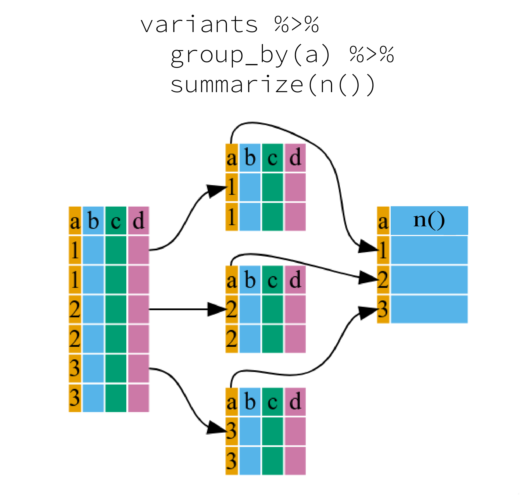
^[The figure was adapted from the Software Carpentry lesson, R for Reproducible Scientific Analysis]
Here the summary function used was n() to find the count for each
group. Since this is a quite a common operation, there is a simpler method
called tally():
variants %>%
  group_by(sample_id) %>%
  tally()
# A tibble: 3 x 2
  sample_id      n
  <chr>      <int>
1 SRR2584863    25
2 SRR2584866   766
3 SRR2589044    10
To show that there are many ways to acheive the same results, there is another way to appraoch this, which bypasses group_by() using the function count():
variants %>%
  count(sample_id)
# A tibble: 3 x 2
  sample_id      n
  <chr>      <int>
1 SRR2584863    25
2 SRR2584866   766
3 SRR2589044    10
We can also apply many other functions to individual columns to get other
summary statistics. For example,we can use built-in functions like mean(),
median(), min(), and max(). These are called “built-in functions” because
they come with R and don’t require that you install any additional packages.
By default, all R functions operating on vectors that contains missing data will return NA.
It’s a way to make sure that users know they have missing data, and make a
conscious decision on how to deal with it. When dealing with simple statistics
like the mean, the easiest way to ignore NA (the missing data) is
to use na.rm = TRUE (rm stands for remove).
So to view the highest filtered depth (DP) for each sample:
variants %>%
  group_by(sample_id) %>%
  summarize(max(DP))
# A tibble: 3 x 2
  sample_id  `max(DP)`
  <chr>          <dbl>
1 SRR2584863        20
2 SRR2584866        79
3 SRR2589044        16
Much of this lesson was copied or adapted from Jeff Hollister’s materials
Key Points
Use the
dplyrpackage to manipulate data frames.Use
glimpse()to quickly look at your data frame.Use
select()to choose variables from a data frame.Use
filter()to choose data based on values.Use
mutate()to create new variables.Use
group_by()andsummarize()to work with subsets of data.