Introducing R and RStudio IDE
Overview
Teaching: 30 min
Exercises: 15 minQuestions
Why use R?
Why use RStudio and how does it differ from R?
Objectives
Know advantages of analyzing data in R
Know advantages of using RStudio
Create an RStudio project, and know the benefits of working within a project
Be able to customize the RStudio layout
Be able to locate and change the current working directory with
getwd()andsetwd()Compose an R script file containing comments and commands
Understand what an R function is
Locate help for an R function using
?,??, andargs()
Getting ready to use R for the first time
In this lesson we will take you through the very first things you need to get R working.
A Brief History of R
R has been around since 1995, and was created by Ross Ihaka and Robert Gentleman at the University of Auckland, New Zealand. R is based off the S programming language developed at Bell Labs and was developed to teach intro statistics. See this slide deck by Ross Ihaka for more info on the subject.
Advantages of using R
At more than 20 years old, R is fairly mature and growing in popularity. However, programming isn’t a popularity contest. Here are key advantages of analyzing data in R:
-
R is open source. This means R is free - an advantage if you are at an institution where you have to pay for your own MATLAB or SAS license. Open source, is important to your colleagues in parts of the world where expensive software is inaccessible. Being open source it also means that R is actively developed by a community (see r-project.org), and there are regular updates.
-
R is widely used. Ok, maybe programming is a popularity contest. Because, R is used in many areas (not just bioinformatics), you are more likely to find help online when you need it. Chances are, almost any error message you run into, someone else has already experienced.
-
R is powerful. R runs on multiple platforms (Windows/MacOS/Linux). It can work with much larger datasets than popular spreadsheet programs like Microsoft Excel, and because of its scripting capabilities is far more reproducible. Also, there are thousands of available software packages for science, including genomics and other areas of life science.
Discussion: Your experience
What has motivated you to learn R? Have you had a research question for which spreadsheet programs such as Excel have proven difficult to use, or where the size of the data set created issues?
Introducing RStudio
In these lessons, we will be making use of a software called RStudio, an Integrated Development Environment (IDE). RStudio, like most IDEs, provides a graphical interface to R, making it more user-friendly, and providing dozens of useful features. We will introduce additional benefits of using RStudio as you cover the lessons.
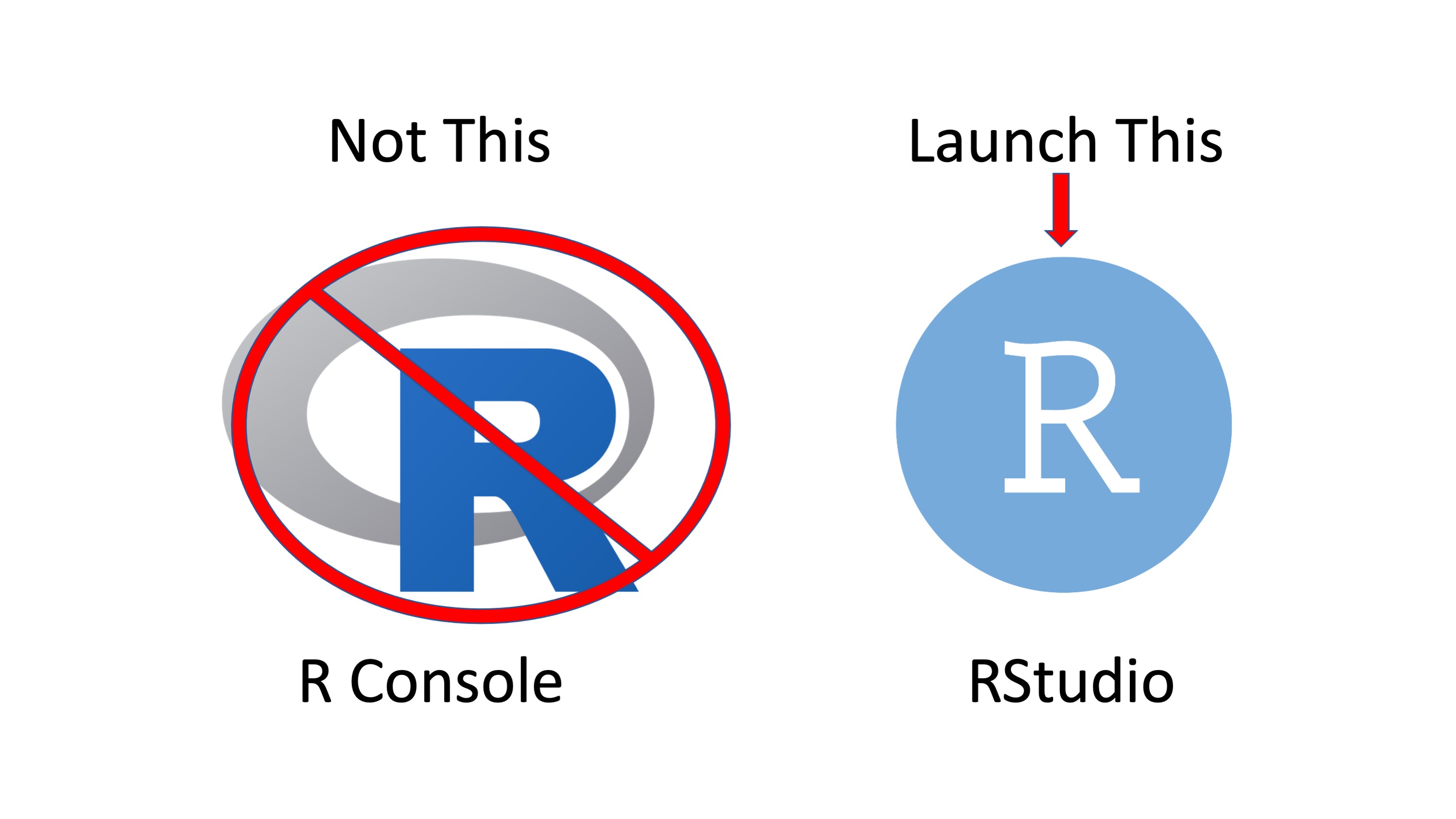
What about this R app should I use that?
Depending on what operating system youre using you will notice in your programs or application menu that there is R Studio and another software that is also R. Currently application icons look like this:
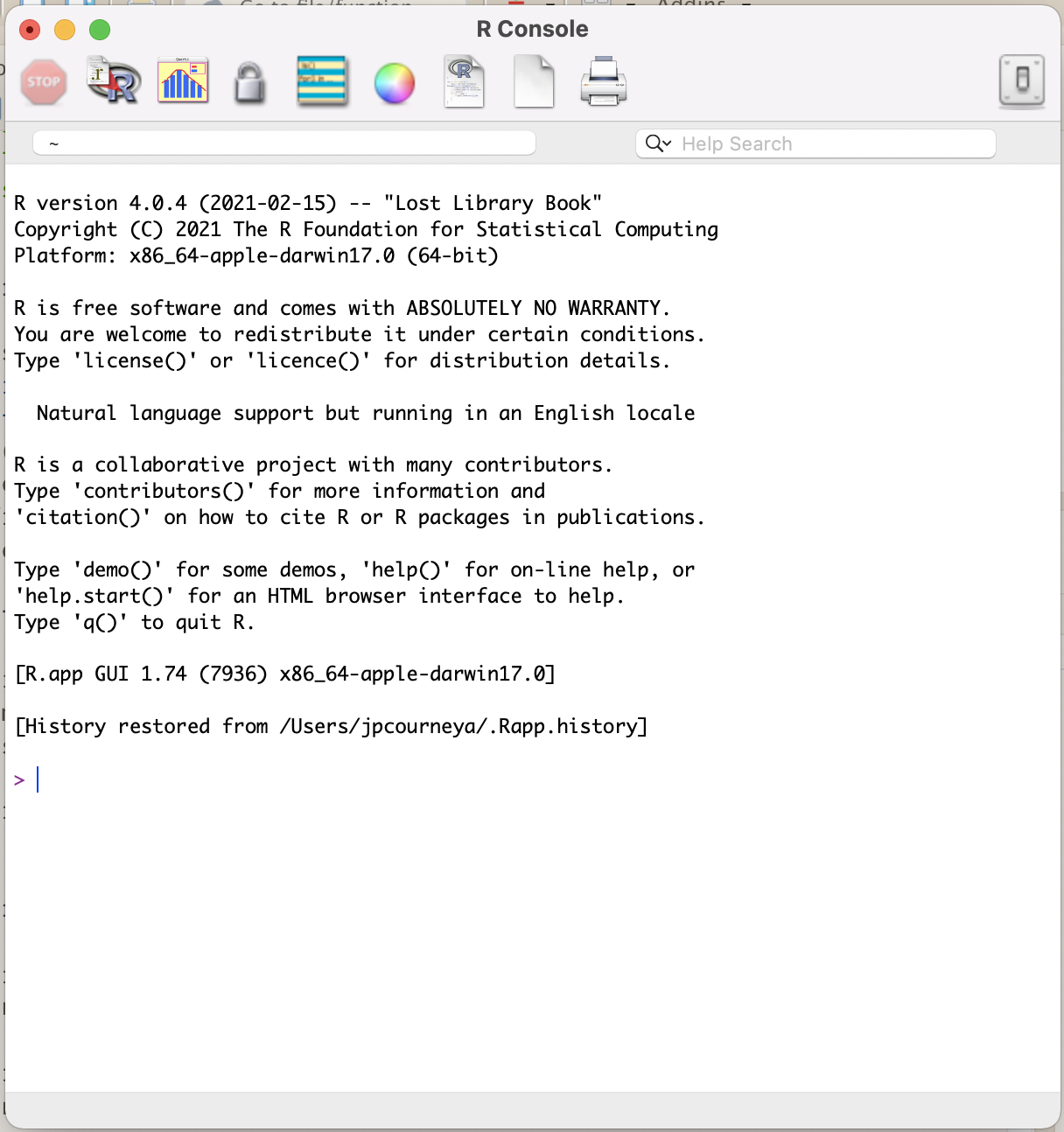
In case you end up launching R and not R Studio you will see an application window that looks like this:
Go ahead and close it out. While there is nothing inherently wrong with using this. The features and benefits RStudio provides for programming in R significantly outweigh those of using the R console. Its recommended that you use RStudio.
Overview and customization of the RStudio layout
Here are the major windows (or panes) of the RStudio environment:
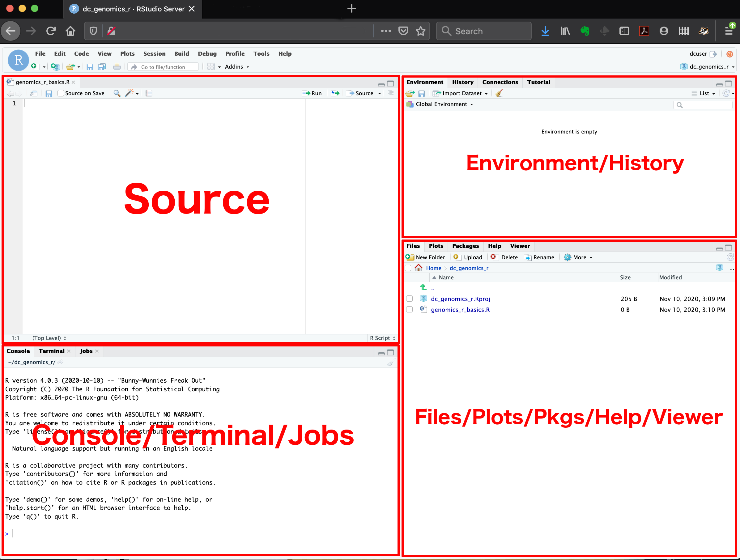
- Source: This pane is where you will write/view R scripts. Some outputs
(such as if you view a dataset using
View()) will appear as a tab here. - Console/Terminal/Jobs: This is actually where you see the execution of commands. This is the same display you would see if you were using R at the command line without RStudio. You can work interactively (i.e. enter R commands here), but for the most part we will run a script (or lines in a script) in the source pane and watch their execution and output here. The “Terminal” tab give you access to the BASH terminal (the Linux operating system, unrelated to R). RStudio also allows you to run jobs (analyses) in the background. This is useful if some analysis will take a while to run. You can see the status of those jobs in the background.
- Environment/History: Here, RStudio will show you what datasets and objects (variables) you have created and which are defined in memory. You can also see some properties of objects/datasets such as their type and dimensions. The “History” tab contains a history of the R commands you’ve executed R.
- Files/Plots/Packages/Help/Viewer: This multipurpose pane will show you the contents of directories on your computer. You can also use the “Files” tab to navigate and set the working directory. The “Plots” tab will show the output of any plots generated. In “Packages” you will see what packages are actively loaded, or you can attach installed packages. “Help” will display help files for R functions and packages. “Viewer” will allow you to view local web content (e.g. HTML outputs).
All of the panes in RStudio have configuration options. For example, you can minimize/maximize a pane, or by moving your mouse in the space between panes you can resize as needed. The most important customization options for pane layout are in the View menu. Other options such as font sizes, colors/themes, and more are in the Tools menu under Global Options.
You are working with R
Although we won’t be working with R at the terminal, there are lots of reasons to. For example, once you have written an RScript, you can run it at any Linux or Windows terminal without the need to start up RStudio. We don’t want you to get confused - RStudio runs R, but R is not RStudio. For more on running an R Script at the terminal see this Software Carpentry lesson.
Create an RStudio project
One of the first benefits we will take advantage of in RStudio is something called an RStudio Project. An RStudio project allows you to more easily:
- Save data, files, variables, packages, etc. related to a specific analysis project
- Restart work where you left off
- Collaborate, especially if you are using version control such as git.
-
To create a project, go to the File menu, and click New Project....
-
In the window that opens select New Directory, then New Project. For “Directory name:” enter post-docs_genomics_r. For “Create project as subdirectory of”, click Browse... and then click Choose which will select your
DocumentsorDesktopdirectory. -
Finally click Create Project. In the “Files” tab of your output pane (more about the RStudio layout in a moment), you should see an RStudio project file, post-docs_genomics_r.Rproj. All RStudio projects end with the “.Rproj” file extension.
Now when we start R in this project directory, or open this project with RStudio, all of our work on this project will be entirely self-contained in this directory.
Best practices for project organization
Although there is no “best” way to lay out a project, there are some general principles to adhere to that will make project management easier:
Treat data as read only
This is probably the most important goal of setting up a project. Data is typically time consuming and/or expensive to collect. Working with them interactively (e.g., in Excel) where they can be modified means you are never sure of where the data came from, or how it has been modified since collection. It is therefore a good idea to treat your data as “read-only”.
Data Cleaning
In many cases your data will be “dirty”: it will need significant preprocessing to get into a format R (or any other programming language) will find useful. This task is sometimes called “data munging”. I find it useful to store these scripts in a separate folder, and create a second “read-only” data folder to hold the “cleaned” data sets.
Treat generated output as disposable
Anything generated by your scripts should be treated as disposable: it should all be able to be regenerated from your scripts.
There are lots of different ways to manage this output. I find it useful to have an output folder with different sub-directories for each separate analysis. This makes it easier later, as many of my analyses are exploratory and don’t end up being used in the final project, and some of the analyses get shared between projects.
Tip: Good Enough Practices for Scientific Computing
Good Enough Practices for Scientific Computing gives the following recommendations for project organization:
- Put each project in its own directory, which is named after the project.
- Put text documents associated with the project in the
docdirectory.- Put raw data and metadata in the
datadirectory, and files generated during cleanup and analysis in aresultsdirectory.- Put source for the project’s scripts and programs in the
srcdirectory, and programs brought in from elsewhere or compiled locally in thebindirectory.- Name all files to reflect their content or function.
Now that you have been presented some practices to keep your data projects in R organized lets put the practice in to action.
Exercise: Create sub-directories for your project.
A) Create a
docdirectory to store text documents.B) Create a
datadirectory for raw data and metadataC) Create a
resultsdirectory for files generated during cleanup and analysisD) Create a
srcdirectory for your scripts.Solution
A) Using the RStudio Files tab in
pane 4click the New Folder button. We will call the folder:docB) Using the RStudio Files tab in
pane 4click the New Folder button. We will call the folder:dataC) Using the RStudio Files tab in
pane 4click the New Folder button. We will call the folder:resultsD) Using the RStudio Files tab in
pane 4click the New Folder button. We will call the folder:src
Save some data in the data directory
Now we have a good directory structure we will now place/save data files in the data/ directory.
Challenge 1
Download the
combined_tidy_vcfdata from here.
- Download the file
- Make sure it’s saved under the name
combined_tidy_vcf.csv- Save the file in the
data/folder within your project.We will load and inspect these data later.
Creating your first R script
Now that we are ready to start exploring R, we will want to keep a record of the commands we are using. To do this we can create an R script:
Click the File menu and select New File and then R Script. Before we go any further, save your script by clicking the save/disk icon that is in the bar above the first line in the script editor, or click the File menu and select save. In the “Save File” window that opens, name your file “genomics_r_basics”. The new script genomics_r_basics.R should appear under “files” in the output pane. By convention, R scripts end with the file extension .R.
Getting to work with R: navigating directories
Now that we have covered the more aesthetic aspects of RStudio, we can get to work using some commands. We will write, execute, and save the commands we learn in our genomics_r_basics.R script that is loaded in the Source pane. First, lets see what directory we are in. To do so, type the following command into the script:
getwd()
To execute this command, make sure your cursor is on the same line the command is written. Then click the Run button that is just above the first line of your script in the header of the Source pane.
In the console, we expect to see the following output:
[1] "~/Documents/post-docs_genomics_r"
* Notice, at the Console, you will also see the instruction you executed above the output in blue.
Since we will be learning several commands, we may already want to keep some
short notes in our script to explain the purpose of the command. Entering a # , or using the keyboard short cut Cntrl + Shift + C, before any line in an R script turns that line into a comment, which R will not try to interpret as code. Edit your script to include a comment on the purpose of commands you are learning, e.g.:
# this command shows the current working directory
getwd()
Exercise: Work interactively in R
What happens when you try to enter the
getwd()command in the Console pane?Solution
You will get the same output you did as when you ran
getwd()from the source. You can run any command in the Console, however, executing it from the source script will make it easier for us to record what we have done, and ultimately run an entire script, instead of entering commands one-by-one.
Next, lets create a folder in Documents or Desktop using the RStudio Files tab in pane 4 using the New Folder button. We will call the folder: R_data.
For the purposes of this exercise we want you to be in the directory "~/Documents/R_data". What if you weren’t? You can set your working directory using the setwd() command. Enter this command in your script, but don’t run this yet.
# This sets the working directory
setwd()
You may have guessed, you need to tell the setwd() command
what directory you want to set as your working directory. To do so, inside of the parentheses, open a set of quotes. Inside the quotes enter a ~/ which is the home directory for Linux, Mac and Windows. Next, use the Tab key, to take advantage of RStudio’s Tab-autocompletion method, to select Documents or Desktop depending on what you designated,
and the new folder R_data you just created. The path in your script should look like this:
# This sets the working directory
setwd("~/Documents/R_data")
When you run this command, the console repeats the command, but gives you no
output. Instead, you see the blank R prompt: >. Congratulations! Although it
seems small, knowing what your working directory is and being able to set your
working directory is the first step to analyzing your data.
Tip: Never use
setwd()Wait, what was the last 2 minutes about? Well, setting your working directory is something you need to do, you need to be very careful about using this as a step in your script. For example, what if your script is being on a computer that has a different directory structure? The top-level path in a Unix file system is root
/, but on Windows it is likelyC:\. This is one of several ways you might cause a script to break because a file path is configured differently than your script anticipates. R packages like here and file.path allow you to specify file paths is a way that is more operating system independent. See Jenny Bryan’s blog post for this and other R tips.
Exercise
Use
setwd()to set the working directory back to the project directory you created in the “Create and RStudio Project” section.Solution
In your script write
setwd("~/Documents/post-docs_genomics_r")orsetwd("~/Desktop/post-docs_genomics_r")and hit Control + Enter. You can also write that in the console. Notice that you need to provide an absolute path to the directory/folder you are going to set the working directory to.Alternatively you can use the Files tab in
pane 4to navigate to your project folder, when there click the More/Gear Icon then selectSet as Working Directory
Using functions in R, without needing to master them
A function in R (or any computing language) is a short
program that takes some input and returns some output. Functions may seem like an advanced topic (and they are), but you have already
used at least one function in R. getwd() is a function! The next sections will help you understand what is happening in
any R script.
Exercise: What do these functions do?
Try the following functions by writing them in your script. See if you can guess what they do, and make sure to add comments to your script about your assumed purpose.
dir()sessionInfo()date()Sys.time()Solution
dir()# Lists files in the working directorysessionInfo()# Gives the version of R and additional info including on attached packagesdate()# Gives the current dateSys.time()# Gives the current timeNotice: Commands are case sensitive!
You have hopefully noticed a pattern - an R function has three key properties:
- Functions have a name (e.g.
dir,getwd); note that functions are case sensitive! - Following the name, functions have a pair of
() - Inside the parentheses, a function may take 0 or more arguments
An argument may be a specific input for your function and/or may modify the
function’s behavior. For example the function round() will round a number
with a decimal:
# This will round a number to the nearest integer
round(3.14)
[1] 3
Getting help with function arguments
What if you wanted to round to one significant digit? round() can
do this, but you may first need to read the help to find out how. To see the help
(In R sometimes also called a “vignette”) enter a ? in front of the function
name:
?round()
The Help tab in pane 4 will show you information (often, too much information). You
will slowly learn how to read and make sense of help files. Checking the “Usage” or “Examples”
headings is often a good place to look first. If you look under “Arguments,” we
also see what arguments we can pass to this function to modify its behavior.
You can also see a function’s argument using the args() function:
args(round)
function (x, digits = 0)
NULL
round() takes two arguments, x, which is the number to be
rounded, and a
digits argument. The = sign indicates that a default (in this case 0) is
already set. Since x is not set, round() requires we provide it, in contrast
to digits where R will use the default value 0 unless you explicitly provide
a different value. We can explicitly set the digits parameter when we call the
function:
round(3.14159, digits = 2)
[1] 3.14
Or, R accepts what we call “positional arguments”, if you pass a function
arguments separated by commas, R assumes that they are in the order you saw
when we used args(). In the case below that means that x is 3.14159 and
digits is 2.
round(3.14159, 2)
[1] 3.14
Finally, what if you are using ? to get help for a function in a package not installed on your system, such as when you are running a script which has dependencies.
?geom_point()
will return an error:
Error in .helpForCall(topicExpr, parent.frame()) :
   no methods for ‘geom_point’ and no documentation for it as a function
Use two question marks (i.e. ??geom_point()) and R will return
results from a search of the documentation for packages you have installed on your computer
in the “Help” tab. Finally, if you think there
should be a function, for example a statistical test, but you aren’t
sure what it is called in R, or what functions may be available, use
the help.search() function.
Exercise: Searching for R functions
Use
help.search()to find R functions for the following statistical functions. Remember to put your search query in quotes inside the function’s parentheses.
- Chi-Squared test
- Student-t test
- mixed linear model
Solution
While your search results may return several tests, we list a few you might find:
- Chi-Squared test:
stats::Chisquare- Student-t test:
stats::TDist- mixed linear model:
stats::lm.glm
We will discuss more on where to look for the libraries and packages that contain functions you want to use. For now, be aware that two important ones are CRAN - the main repository for R, and Bioconductor - a popular repository for bioinformatics-related R packages which we will learn more about later.
RStudio contextual help
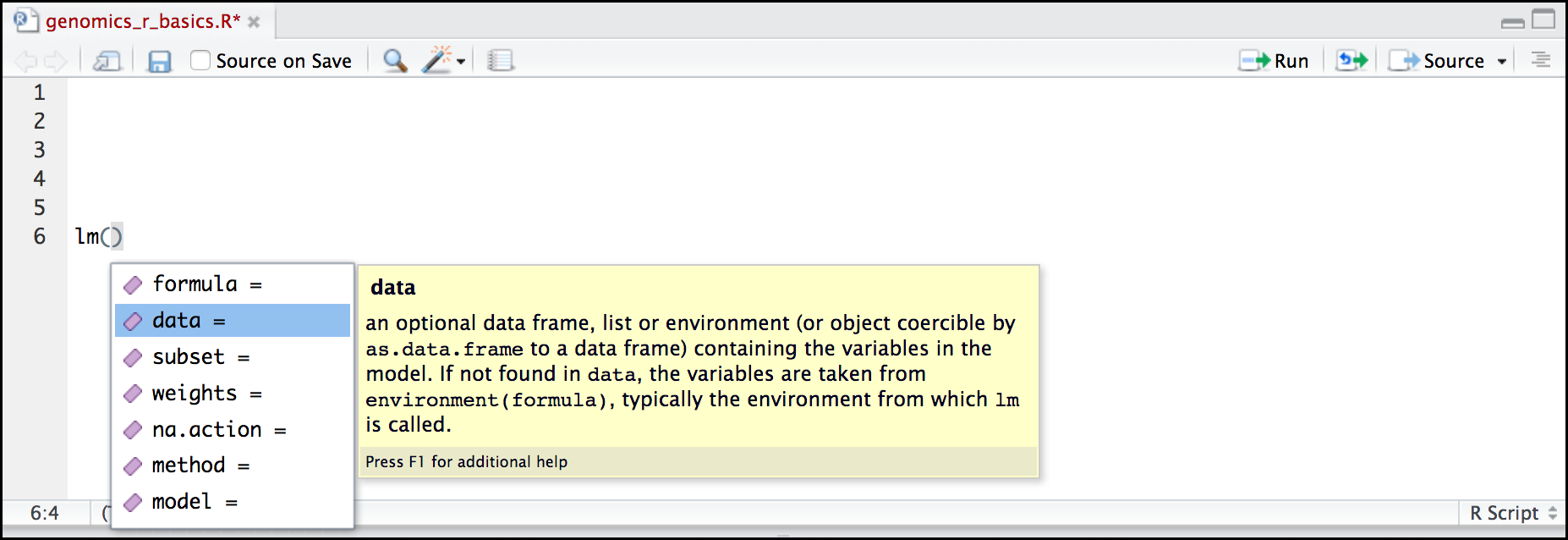
Here is one last bonus we will mention about RStudio. It’s difficult to remember all of the arguments and definitions associated with a given function. When you start typing the name of a function and hit the Tab key, RStudio will display functions and associated help:
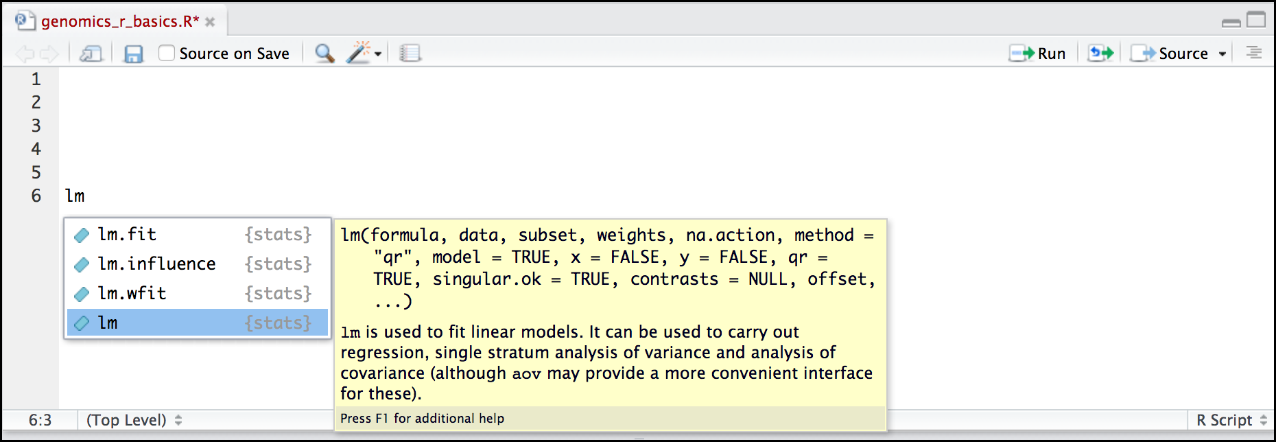
Once you type a function, hitting the Tab inside the parentheses will show you the function’s arguments and provide additional help for each of these arguments.
When you have no idea where to begin
If you don’t know what function or package you need to use CRAN Task Views is a specially maintained list of packages grouped into fields. This can be a good starting point.
When your code doesn’t work: seeking help from your peers
If you’re having trouble using a function, 9 times out of 10,
the answers you are seeking have already been answered on
Stack Overflow. You can search using
the [r] tag. You can also Google it which typically takes you to a Stack Overflow post.
If you can’t find the answer, there are a few useful functions to help you ask a question from your peers:
?dput
Will dump the data you’re working with into a format so that it can be copy and pasted by anyone else into their R session.
sessionInfo()
R version 4.0.4 (2021-02-15)
Platform: x86_64-apple-darwin17.0 (64-bit)
Running under: macOS Big Sur 10.16

Matrix products: default
BLAS:   /Library/Frameworks/R.framework/Versions/4.0/Resources/lib/libRblas.dylib
LAPACK: /Library/Frameworks/R.framework/Versions/4.0/Resources/lib/libRlapack.dylib

locale:
[1] en_US.UTF-8/en_US.UTF-8/en_US.UTF-8/C/en_US.UTF-8/en_US.UTF-8

attached base packages:
[1] stats     graphics  grDevices utils     datasets  methods   base

other attached packages:
[1] knitr_1.33

loaded via a namespace (and not attached):
[1] compiler_4.0.4 magrittr_2.0.1 tools_4.0.4    stringi_1.7.3  stringr_1.4.0
[6] xfun_0.24      evaluate_0.14
Will print out your current version of R, as well as any packages you have loaded. This can be useful for others to help reproduce and debug your issue.
Other ports of call
Key Points
R is a powerful, popular open-source scripting language
You can customize the layout of RStudio, and use the project feature to manage the files and packages used in your analysis
RStudio allows you to run R in an easy-to-use interface and makes it easy to find help
R Basics
Overview
Teaching: 60 min
Exercises: 20 minQuestions
What will these lessons not cover?
What are the basic features of the R language?
What are the most common objects in R?
Objectives
Be able to create the most common R objects including vectors
Understand that vectors have modes, which correspond to the type of data they contain
Be able to use arithmetic operators on R objects
Be able to retrieve (subset), name, or replace, values from a vector
Be able to use logical operators in a subsetting operation
Understand that lists can hold data of more than one mode and can be indexed
“The fantastic world of R awaits you” OR “Nobody wants to learn how to use R”
Before we begin this lesson, we want you to be clear on the goal of the workshop and these lessons. We believe that every learner can achieve competency with R.
You have reached competency when you find that you are able to use R to handle common analysis challenges in a reasonable amount of time (which includes time needed to look at learning materials, search for answers online, and ask colleagues for help). As you spend more time using R (there is no substitute for regular use and practice) you will find yourself gaining competency and even expertise. The more familiar you get, the more complex the analyses you will be able to carry out, with less frustration, and in less time - the fantastic world of R awaits you!
What these lessons will not teach you
Nobody wants to learn how to use R. People want to learn how to use R to analyze their own research questions!
Ok, maybe some folks learn R for R’s sake, but these lessons assume that you want to start analyzing genomic data as soon as possible. Given this, there are many valuable pieces of information about R that we simply won’t have time to cover. Hopefully, we will clear the hurdle of giving you just enough knowledge to be dangerous, which can be a high bar in R! We suggest you look into the additional learning materials in the tip box below.
Here are some R skills we will not cover in these lessons
-
How to create and work with R matrices and R lists
-
How to create and work with loops and conditional statements, and the “apply” family of functions (which are super useful, read more here)
-
How to do basic string manipulations (e.g. finding patterns in text using grep, replacing text)
-
How to plot using the default R graphic tools (we will cover plot creation, but will do so using the popular plotting package
ggplot2) -
How to use advanced R statistical functions
Tip: Where to learn more
The following are good resources for learning more about R. Some of them can be quite technical, but if you are a regular R user you may ultimately need this technical knowledge.
- R for Beginners: By Emmanuel Paradis and a great starting point
- The R Manuals: Maintained by the R project
- R contributed documentation: Also linked to the R project; importantly there are materials available in several languages
- R for Data Science: A wonderful collection by noted R educators and developers Garrett Grolemund and Hadley Wickham
- Practical Data Science for Stats: Not exclusively about R usage, but a nice collection of pre-prints on data science and applications for R
- Programming in R Software Carpentry lesson: There are several Software Carpentry lessons in R to choose from
Creating objects in R
Reminder
At this point you should be coding along in the “genomics_r_basics.R” script we created in the last episode. Writing your commands in the script (and commenting it) will make it easier to record what you did and why.
What might be called a variable in many languages is called an object in R.
To create an object you need:
-
a name (e.g. ‘a’)
-
a value (e.g. ‘1’)
-
the assignment operator (‘<-‘)
In your script, “genomics_r_basics.R”, using the R assignment operator ‘<-‘, assign ‘1’ to the object ‘a’ as shown. Remember to leave a comment in the line above (using the ‘#’) to explain what you are doing:
# this line creates the object 'a' and assigns it the value '1'

a <- 1
Next, run this line of code in your script. You can run a line of code by hitting the Run button that is just above the first line of your script in the header of the Source pane or you can use the appropriate shortcut:
- Windows execution shortcut: Ctrl+Enter
- Mac execution shortcut: Cmd(⌘)+Enter
To run multiple lines of code, you can highlight all the line you wish to run and then hit Run or use the shortcut key combo listed above.
In the RStudio ‘Console’ you should see:
a <- 1
>
The ‘Console’ will display lines of code run from a script and any outputs or status/warning/error messages (usually in red).
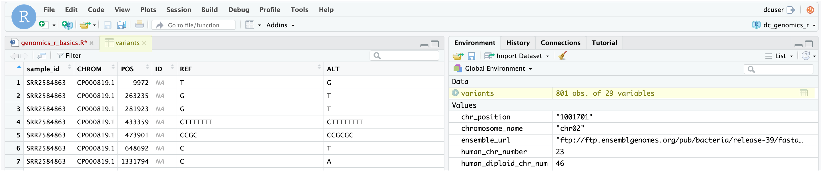
In the ‘Environment’ window you will also get a table:

The ‘Environment’ window allows you to keep track of the objects you have created in R.
Exercise: Create some objects in R
Create the following objects; give each object an appropriate name (your best guess at what name to use is fine):
- Create an object that has the value of number of pairs of human chromosomes
- Create an object that has a value of your favorite gene name
- Create an object that has this URL as its value: “ftp://ftp.ensemblgenomes.org/pub/bacteria/release-39/fasta/bacteria_5_collection/escherichia_coli_b_str_rel606/”
- Create an object that has the value of the number of chromosomes in a diploid human cell
Solution
Here as some possible answers to the challenge:
human_chr_number <- 23
gene_name <- 'pten'
ensemble_url <- 'ftp://ftp.ensemblgenomes.org/pub/bacteria/release-39/fasta/bacteria_5_collection/escherichia_coli_b_str_rel606/'
human_diploid_chr_num <-  2 * human_chr_number
Naming objects in R
Here are some important details about naming objects in R.
- Avoid spaces and special characters: Object names cannot contain spaces or the minus sign (
-). You can use ‘_’ to make names more readable. You should avoid using special characters in your object name (e.g. ! @ # . , etc.). Also, object names cannot begin with a number. - Use short, easy-to-understand names: You should avoid naming your objects using single letters (e.g. ‘n’, ‘p’, etc.). This is mostly to encourage you to use names that would make sense to anyone reading your code (a colleague, or even yourself a year from now). Also, avoiding excessively long names will make your code more readable.
- Avoid commonly used names: There are several names that may already have a definition in the R language (e.g. ‘mean’, ‘min’, ‘max’). One clue that a name already has meaning is that if you start typing a name in RStudio and it gets a colored highlight or RStudio gives you a suggested autocompletion you have chosen a name that has a reserved meaning.
- Use the recommended assignment operator: In R, we use ‘<- ‘ as the
preferred assignment operator. ‘=’ works too, but is most commonly used in
passing arguments to functions (more on functions later). There is a shortcut
for the R assignment operator:
- Windows execution shortcut: Alt+-
- Mac execution shortcut: Option+-
There are a few more suggestions about naming and style you may want to learn more about as you write more R code. There are several “style guides” that have advice, and one to start with is the tidyverse R style guide.
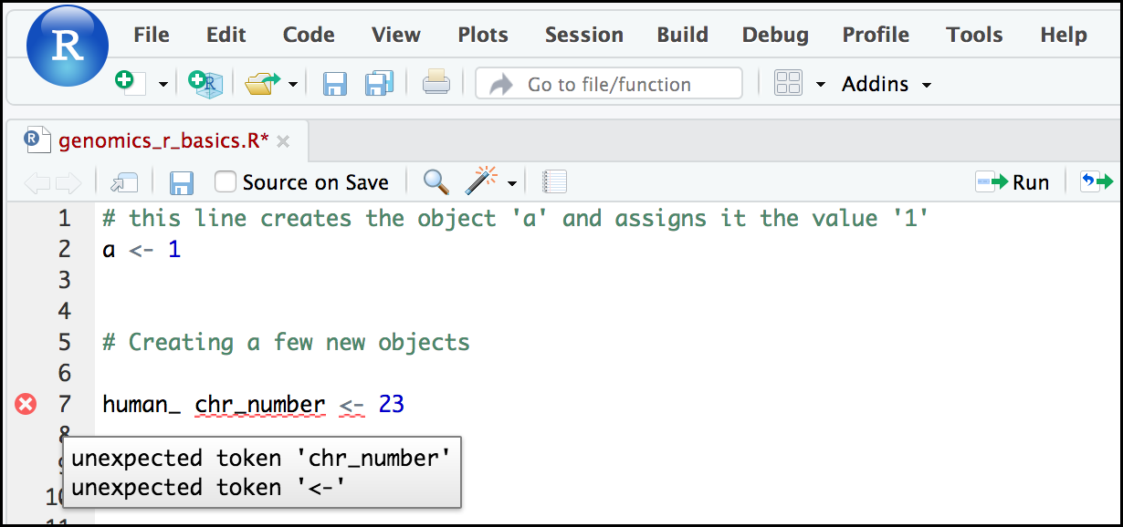
Tip: Pay attention to warnings in the script console
If you enter a line of code in your script that contains an error, RStudio may give you an error message and underline this mistake. Sometimes these messages are easy to understand, but often the messages may need some figuring out. Paying attention to these warnings will help you avoid mistakes. In the example below, our object name has a space, which is not allowed in R. The error message does not say this directly, but R is “not sure” about how to assign the name to “human_ chr_number” when the object name we want is “human_chr_number”.
Reassigning object names or deleting objects
Once an object has a value, you can change that value by overwriting it. R will not give you a warning or error if you overwriting an object, which may or may not be a good thing depending on how you look at it.
# gene_name has the value 'pten' or whatever value you used in the challenge.
# We will now assign the new value 'tp53'
gene_name <- 'tp53'
You can also remove an object from R’s memory entirely. The rm() function
will delete the object.
# delete the object 'gene_name'
rm(gene_name)
If you run a line of code that has only an object name, R will normally display the contents of that object. In this case, we are told the object no longer exists.
Error: object 'gene_name' not found
Understanding object data types (modes)
In R, every object has two properties:
- Length: How many distinct values are held in that object
- Mode: What is the classification (type) of that object.
We will get to the “length” property later in the lesson. The “mode” property corresponds to the type of data an object represents. The most common modes you will encounter in R are:
| Mode (abbreviation) | Type of data |
|---|---|
| Numeric (num) | Numbers such floating point/decimals (1.0, 0.5, 3.14), there are also more specific numeric types (dbl - Double, int - Integer). These differences are not relevant for most beginners and pertain to how these values are stored in memory |
| Character (chr) | A sequence of letters/numbers in single ‘’ or double “ “ quotes |
| Logical | Boolean values - TRUE or FALSE |
There are a few other modes (i.e. “complex”, “raw” etc.) but these are the three we will work with in this lesson.
Data types are familiar in many programming languages, but also in natural language where we refer to them as the parts of speech, e.g. nouns, verbs, adverbs, etc. Once you know if a word - perhaps an unfamiliar one - is a noun, you can probably guess you can count it and make it plural if there is more than one (e.g. 1 Tuatara, or 2 Tuataras). If something is a adjective, you can usually change it into an adverb by adding “-ly” (e.g. jejune vs. jejunely). Depending on the context, you may need to decide if a word is in one category or another (e.g “cut” may be a noun when it’s on your finger, or a verb when you are preparing vegetables). These concepts have important analogies when working with R objects.
Exercise: Create objects and check their modes
Create the following objects in R, then use the
mode()function to verify their modes. Try to guess what the mode will be before you look at the solution
chromosome_name <- 'chr02'od_600_value <- 0.47chr_position <- '1001701'spock <- TRUEpilot <- EarhartSolution
Error in eval(expr, envir, enclos): object 'Earhart' not foundmode(chromosome_name)[1] "character"mode(od_600_value)[1] "numeric"mode(chr_position)[1] "character"mode(spock)[1] "logical"mode(pilot)Error in mode(pilot): object 'pilot' not found
Notice from the solution that even if a series of numbers is given as a value
R will consider them to be in the “character” mode if they are enclosed as
single or double quotes. Also, notice that you cannot take a string of alphanumeric
characters (e.g. Earhart) and assign as a value for an object. In this case,
R looks for an object named Earhart but since there is no object, no assignment can
be made. If Earhart did exist, then the mode of pilot would be whatever
the mode of Earhart was originally. If we want to create an object
called pilot that was the name “Earhart”, we need to enclose
Earhart in quotation marks.
pilot <- "Earhart"
mode(pilot)
[1] "character"
Mathematical and functional operations on objects
Once an object exists (which by definition also means it has a mode), R can appropriately manipulate that object. For example, objects of the numeric modes can be added, multiplied, divided, etc. R provides several mathematical (arithmetic) operators including:
| Operator | Description |
|---|---|
| + | addition |
| - | subtraction |
| * | multiplication |
| / | division |
| ^ or ** | exponentiation |
| a%/%b | integer division (division where the remainder is discarded) |
| a%%b | modulus (returns the remainder after division) |
These can be used with literal numbers:
(1 + (5 ** 0.5))/2
[1] 1.618034
and importantly, can be used on any object that evaluates to (i.e. interpreted by R) a numeric object:
# multiply the object 'human_chr_number' by 2

human_chr_number * 2
[1] 46
Exercise: Compute the golden ratio
One approximation of the golden ratio (φ) can be found by taking the sum of 1 and the square root of 5, and dividing by 2 as in the example above. Compute the golden ratio to 3 digits of precision using the
sqrt()andround()functions. Hint: remember theround()function can take 2 arguments.Solution
round((1 + sqrt(5))/2, digits = 3)[1] 1.618Notice that you can place one function inside of another.
Vectors
Vectors are probably the most commonly used object type in R.
A vector is a collection of values that are all of the same type (numbers, characters, etc.).
One of the most common ways to create a vector is to use the c() function - the “concatenate” or “combine” function. Inside the function you may enter one or more values; for multiple values, separate each value with a comma:
# Create the SNP gene name vector

snp_genes <- c("OXTR", "ACTN3", "AR", "OPRM1")
Vectors always have a mode and a length.
You can check these with the mode() and length() functions respectively.
A useful function that gives both of these pieces of information is the
str() (structure) function.
# Check the mode, length, and structure of 'snp_genes'
mode(snp_genes)
[1] "character"
length(snp_genes)
[1] 4
str(snp_genes)
chr [1:4] "OXTR" "ACTN3" "AR" "OPRM1"
Vectors are quite important in R. Another data type that we will work with later in this lesson, data frames, are collections of vectors. What we learn here about vectors will pay off even more when we start working with data frames.
Creating and subsetting vectors
Let’s create a few more vectors to play around with:
# Some interesting human SNPs
# while accuracy is important, typos in the data won't hurt you here

snps <- c('rs53576', 'rs1815739', 'rs6152', 'rs1799971')
snp_chromosomes <- c('3', '11', 'X', '6')
snp_positions <- c(8762685, 66560624, 67545785, 154039662)
Once we have vectors, one thing we may want to do is specifically retrieve one or more values from our vector. To do so, we use bracket notation. We type the name of the vector followed by square brackets. In those square brackets we place the index (e.g. a number) in that bracket as follows:
# get the 3rd value in the snp_genes vector
snp_genes[3]
[1] "AR"
In R, every item your vector is indexed, starting from the first item (1) through to the final number of items in your vector. You can also retrieve a range of numbers:
# get the 1st through 3rd value in the snp_genes vector

snp_genes[1:3]
[1] "OXTR" "ACTN3" "AR"
If you want to retrieve several (but not necessarily sequential) items from a vector, you pass a vector of indices; a vector that has the numbered positions you wish to retrieve.
# get the 1st, 3rd, and 4th value in the snp_genes vector

snp_genes[c(1, 3, 4)]
[1] "OXTR" "AR" "OPRM1"
There are additional (and perhaps less commonly used) ways of subsetting a vector (see these examples). Also, several of these subsetting expressions can be combined:
# get the 1st through the 3rd value, and 4th value in the snp_genes vector
# yes, this is a little silly in a vector of only 4 values.
snp_genes[c(1:3,4)]
[1] "OXTR" "ACTN3" "AR" "OPRM1"
Adding to, removing, or replacing values in existing vectors
Once you have an existing vector, you may want to add a new item to it. To do
so, you can use the c() function again to add your new value:
# add the gene 'CYP1A1' and 'APOA5' to our list of snp genes
# this overwrites our existing vector
snp_genes <- c(snp_genes, "CYP1A1", "APOA5")
We can verify that “snp_genes” contains the new gene entry
snp_genes
[1] "OXTR" "ACTN3" "AR" "OPRM1" "CYP1A1" "APOA5"
Using a negative index will return a version of a vector with that index’s value removed:
snp_genes[-6]
[1] "OXTR" "ACTN3" "AR" "OPRM1" "CYP1A1"
We can remove that value from our vector by overwriting it with this expression:
snp_genes <- snp_genes[-6]
snp_genes
[1] "OXTR" "ACTN3" "AR" "OPRM1" "CYP1A1"
We can also explicitly rename or add a value to our index using double bracket notation:
snp_genes[7]<- "APOA5"
snp_genes
[1] "OXTR" "ACTN3" "AR" "OPRM1" "CYP1A1" NA "APOA5"
Notice in the operation above that R inserts an NA value to extend our vector so that the gene “APOA5” is an index 7. This may be a good or not-so-good thing depending on how you use this.
Exercise: Examining and subsetting vectors
Answer the following questions to test your knowledge of vectors
Which of the following are true of vectors in R?
A) All vectors have a mode or a length
B) All vectors have a mode and a length
C) Vectors may have different lengths
D) Items within a vector may be of different modes
E) You can use thec()to one or more items to an existing vector
F) You can use thec()to add a vector to an exiting vectorSolution
A) False - Vectors have both of these properties
B) True
C) True
D) False - Vectors have only one mode (e.g. numeric, character); all items in
a vector must be of this mode. E) True
F) True
Logical Subsetting
There is one last set of cool subsetting capabilities we want to introduce. It is possible within R to retrieve items in a vector based on a logical evaluation or numerical comparison. For example, let’s say we wanted get all of the SNPs in our vector of SNP positions that were greater than 100,000,000. We could index using the ‘>’ (greater than) logical operator:
snp_positions[snp_positions > 100000000]
[1] 154039662
In the square brackets you place the name of the vector followed by the comparison operator and (in this case) a numeric value. Some of the most common logical operators you will use in R are:
| Operator | Description |
|---|---|
| < | less than |
| <= | less than or equal to |
| > | greater than |
| >= | greater than or equal to |
| == | exactly equal to |
| != | not equal to |
| !x | not x |
| a | b | a or b |
| a & b | a and b |
The magic of programming
The reason why the expression
snp_positions[snp_positions > 100000000]works can be better understood if you examine what the expression “snp_positions > 100000000” evaluates to:snp_positions > 100000000[1] FALSE FALSE FALSE TRUEThe output above is a logical vector, the 4th element of which is TRUE. When you pass a logical vector as an index, R will return the true values:
snp_positions[c(FALSE, FALSE, FALSE, TRUE)][1] 154039662If you have never coded before, this type of situation starts to expose the “magic” of programming. We mentioned before that in the bracket notation you take your named vector followed by brackets which contain an index: named_vector[index]. The “magic” is that the index needs to evaluate to a number. So, even if it does not appear to be an integer (e.g. 1, 2, 3), as long as R can evaluate it, we will get a result. That our expression
snp_positions[snp_positions > 100000000]evaluates to a number can be seen in the following situation. If you wanted to know which index (1, 2, 3, or 4) in our vector of SNP positions was the one that was greater than 100,000,000?We can use the
which()function to return the indices of any item that evaluates as TRUE in our comparison:which(snp_positions > 100000000)[1] 4Why this is important
Often in programming we will not know what inputs and values will be used when our code is executed. Rather than put in a pre-determined value (e.g 100000000) we can use an object that can take on whatever value we need. So for example:
snp_marker_cutoff <- 100000000
snp_positions[snp_positions > snp_marker_cutoff]
[1] 154039662Ultimately, it’s putting together flexible, reusable code like this that gets at the “magic” of programming!
A few final vector tricks
Finally, there are a few other common retrieve or replace operations you may
want to know about. First, you can check to see if any of the values of your
vector are missing (i.e. are NA). Missing data will get a more detailed treatment later,
but the is.NA() function will return a logical vector, with TRUE for any NA
value:
# current value of 'snp_genes':
# chr [1:7] "OXTR" "ACTN3" "AR" "OPRM1" "CYP1A1" NA "APOA5"

is.na(snp_genes)
[1] FALSE FALSE FALSE FALSE FALSE TRUE FALSE
Sometimes, you may wish to find out if a specific value (or several values) is
present a vector. You can do this using the comparison operator %in%, which
will return TRUE for any value in your collection that is in
the vector you are searching:
# current value of 'snp_genes':
# chr [1:7] "OXTR" "ACTN3" "AR" "OPRM1" "CYP1A1" NA "APOA5"

# test to see if "ACTN3" or "APO5A" is in the snp_genes vector
# if you are looking for more than one value, you must pass this as a vector

c("ACTN3","APOA5") %in% snp_genes
[1] TRUE TRUE
Review Exercise 1
What data types/modes are the following vectors?
a.
snps
b.snp_chromosomes
c.snp_positionsSolution
typeof(snps)[1] "character"typeof(snp_chromosomes)[1] "character"typeof(snp_positions)[1] "double"
Review Exercise 2
Add the following values to the specified vectors:
a. To the
snpsvector add: ‘rs662799’
b. To thesnp_chromosomesvector add: 11
c. To thesnp_positionsvector add: 116792991Solution
snps <- c(snps, 'rs662799')
snps
[1] "rs53576" "rs1815739" "rs6152" "rs1799971" "rs662799"snp_chromosomes <- c(snp_chromosomes, "11") # did you use quotes? snp_chromosomes[1] "3" "11" "X" "6" "11"snp_positions <- c(snp_positions, 116792991) snp_positions[1] 8762685 66560624 67545785 154039662 116792991
Review Exercise 3
Make the following change to the
snp_genesvector:Hint: Your vector should look like this in ‘Environment’:
chr [1:7] "OXTR" "ACTN3" "AR" "OPRM1" "CYP1A1" NA "APOA5". If not recreate the vector by running this expression:snp_genes <- c("OXTR", "ACTN3", "AR", "OPRM1", "CYP1A1", NA, "APOA5")a. Create a new version of
snp_genesthat does not contain CYP1A1 and then
b. Add 2 NA values to the end ofsnp_genesSolution
snp_genes <- snp_genes[-5]
snp_genes <- c(snp_genes, NA, NA)
snp_genes
[1] "OXTR" "ACTN3" "AR" "OPRM1" NA "APOA5" NA NA
Review Exercise 4
Using indexing, create a new vector named
combinedthat contains:
- The the 1st value in
snp_genes- The 1st value in
snps- The 1st value in
snp_chromosomes- The 1st value in
snp_positionsSolution
combined <- c(snp_genes[1], snps[1], snp_chromosomes[1], snp_positions[1])
combined
[1] "OXTR" "rs53576" "3" "8762685"
Review Exercise 5
What type of data is
combined?Solution
typeof(combined)[1] "character"
Bonus material: Lists
Lists are quite useful in R, but we won’t be using them in the genomics lessons. That said, you may come across lists in the way that some bioinformatics programs may store and/or return data to you. One of the key attributes of a list is that, unlike a vector, a list may contain data of more than one mode. Learn more about creating and using lists using this nice tutorial. In this one example, we will create a named list and show you how to retrieve items from the list.
# Create a named list using the 'list' function and our SNP examples
# Note, for easy reading we have placed each item in the list on a separate line
# Nothing special about this, you can do this for any multiline commands
# To run this command, make sure the entire command (all 4 lines) are highlighted
# before running
# Note also, as we are doing all this inside the list() function use of the
# '=' sign is good style
snp_data <- list(genes = snp_genes,
                 refference_snp = snps,
                 chromosome = snp_chromosomes,
                 position = snp_positions)
# Examine the structure of the list
str(snp_data)
List of 4
 $ genes         : chr [1:8] "OXTR" "ACTN3" "AR" "OPRM1" ...
 $ refference_snp: chr [1:5] "rs53576" "rs1815739" "rs6152" "rs1799971" ...
 $ chromosome    : chr [1:5] "3" "11" "X" "6" ...
 $ position      : num [1:5] 8.76e+06 6.66e+07 6.75e+07 1.54e+08 1.17e+08
To get all the values for the position object in the list, we use the $ notation:
# return all the values of position object

snp_data$position
[1] 8762685 66560624 67545785 154039662 116792991
To get the first value in the position object, use the [] notation to index:
# return first value of the position object

snp_data$position[1]
[1] 8762685
Key Points
Effectively using R is a journey of months or years. Still you don’t have to be an expert to use R and you can start using and analyzing your data with with about a day’s worth of training
It is important to understand how data are organized by R in a given object type and how the mode of that type (e.g. numeric, character, logical, etc.) will determine how R will operate on that data.
Working with vectors effectively prepares you for understanding how data are organized in R.
R Basics continued - factors and data frames
Overview
Teaching: 60 min
Exercises: 30 minQuestions
How do I get started with tabular data (e.g. spreadsheets) in R?
What are some best practices for reading data into R?
How do I save tabular data generated in R?
Objectives
Explain the basic principle of tidy datasets
Be able to load a tabular dataset using base R functions
Be able to determine the structure of a data frame including its dimensions and the datatypes of variables
Be able to subset/retrieve values from a data frame
Understand how R may coerce data into different modes
Be able to change the mode of an object
Understand that R uses factors to store and manipulate categorical data
Be able to manipulate a factor, including subsetting and reordering
Be able to apply an arithmetic function to a data frame
Be able to coerce the class of an object (including variables in a data frame)
Be able to import data from Excel
Be able to save a data frame as a delimited file
Working with spreadsheets (tabular data)
A substantial amount of the data we work with in genomics will be tabular data, this is data arranged in rows and columns - also known as spreadsheets. We could write a whole lesson on how to work with spreadsheets effectively (actually we did). For our purposes, we want to remind you of a few principles before we work with our first set of example data:
1) Keep raw data separate from analyzed data
This is principle number one because if you can’t tell which files are the original raw data, you risk making some serious mistakes (e.g. drawing conclusion from data which have been manipulated in some unknown way). This is a redundancy but important to review!
2) Keep spreadsheet data Tidy
The simplest principle of Tidy data is that we have one row in our spreadsheet for each observation or sample, and one column for every variable that we measure or report on. As simple as this sounds, it’s very easily violated. Most data scientists agree that significant amounts of their time is spent tidying data for analysis. Read more about data organization in our lesson and in this paper.
3) Trust but verify
Finally, while you don’t need to be paranoid about data, you should have a plan for how you will prepare it for analysis. This a focus of this lesson. You probably already have a lot of intuition, expectations, assumptions about your data - the range of values you expect, how many values should have been recorded, etc. Of course, as the data get larger our human ability to keep track will start to fail (and yes, it can fail for small data sets too). R will help you to examine your data so that you can have greater confidence in your analysis, and its reproducibility.
Tip: Keeping you raw data separate
When you work with data in R, you are not changing the original file you loaded that data from. This is different than (for example) working with a spreadsheet program where changing the value of the cell leaves you one “save”-click away from overwriting the original file. You have to purposely use a writing function (e.g.
write.csv()) to save data loaded into R. In that case, be sure to save the modified data into a new file. More on this later in the lesson.
Importing tabular data into R
There are several ways to import data into R. For our purpose here, we will
focus on using the tools every R installation comes with (so called “base” R) to import a comma-delimited file containing the results of a variant calling workflow.
We will need to load the sheet using a function called read.csv().
Exercise: Review the arguments of the
read.csv()functionBefore using the
read.csv()function, use R’s help feature to answer the following questions.Hint: Entering ‘?’ before the function name and then running that line will bring up the help documentation. Also, when reading this particular help be careful to pay attention to the ‘read.csv’ expression under the ‘Usage’ heading. Other answers will be in the ‘Arguments’ heading.
A) What is the default parameter for ‘header’ in the
read.csv()function?B) What argument would you have to change to read a file that was delimited by semicolons (;) rather than commas?
C) What argument would you have to change to read file in which numbers used commas for decimal separation (i.e. 1,00)?
D) What argument would you have to change to read in only the first 10,000 rows of a very large file?
Solution
A) The
read.csv()function has the argument ‘header’ set to TRUE by default, this means the function always assumes the first row is header information, (i.e. column names)B) The
read.csv()function has the argument ‘sep’ set to “,”. This means the function assumes commas are used as delimiters, as you would expect. Changing this parameter (e.g.sep=";") would now interpret semicolons as delimiters.C) Although it is not listed in the
read.csv()usage,read.csv()is a “version” of the functionread.table()and accepts all its arguments. If you setdec=","you could change the decimal operator. We’d probably assume the delimiter is some other character.D) You can set
nrowto a numeric value (e.g.nrow=10000) to choose how many rows of a file you read in. This may be useful for very large files where not all the data is needed to test some data cleaning steps you are applying.Hopefully, this exercise gets you thinking about using the provided help documentation in R. There are many arguments that exist, but which we wont have time to cover. Look here to get familiar with functions you use frequently, you may be surprised at what you find they can do.
Now, let’s read in the file combined_tidy_vcf.csv which will be located in
~/Documents/post-docs_genomics_r/data/. Call this data variants. The
first argument to pass to our read.csv() function is the file path for our
data. The file path must be in quotes and now is a good time to remember to
use tab autocompletion. If you use tab autocompletion you avoid typos and
errors in file paths. Use it!
## read in a CSV file and save it as 'variants'
# assuming youre in the project home directory too!
variants <- read.csv("data/combined_tidy_vcf.csv")
One of the first things you should notice is that in the Environment window,
you have the variants object, listed as 801 obs. (observations/rows)
of 29 variables (columns). Double-clicking on the name of the object will open
a view of the data in a new tab.
Summarizing, subsetting, and determining the structure of a data frame.
A data frame is the standard way in R to store tabular data. A data fame could also be thought of as a collection of vectors, all of which have the same length. Using only two functions, we can learn a lot about out data frame including some summary statistics as well as well as the “structure” of the data frame. Let’s examine what each of these functions can tell us:
## get summary statistics on a data frame

summary(variants)
  sample_id            CHROM                POS             ID
 Length:801         Length:801         Min.   :   1521   Mode:logical
 Class :character   Class :character   1st Qu.:1115970   NA's:801
 Mode  :character   Mode  :character   Median :2290361
                                       Mean   :2243682
                                       3rd Qu.:3317082
                                       Max.   :4629225

     REF                ALT                 QUAL          FILTER
 Length:801         Length:801         Min.   :  4.385   Mode:logical
 Class :character   Class :character   1st Qu.:139.000   NA's:801
 Mode  :character   Mode  :character   Median :195.000
                                       Mean   :172.276
                                       3rd Qu.:225.000
                                       Max.   :228.000

   INDEL              IDV              IMF               DP
 Mode :logical   Min.   : 2.000   Min.   :0.5714   Min.   : 2.00
 FALSE:700       1st Qu.: 7.000   1st Qu.:0.8824   1st Qu.: 7.00
 TRUE :101       Median : 9.000   Median :1.0000   Median :10.00
                 Mean   : 9.396   Mean   :0.9219   Mean   :10.57
                 3rd Qu.:11.000   3rd Qu.:1.0000   3rd Qu.:13.00
                 Max.   :20.000   Max.   :1.0000   Max.   :79.00
                 NA's   :700      NA's   :700
      VDB                 RPB              MQB              BQB
 Min.   :0.0005387   Min.   :0.0000   Min.   :0.0000   Min.   :0.1153
 1st Qu.:0.2180410   1st Qu.:0.3776   1st Qu.:0.1070   1st Qu.:0.6963
 Median :0.4827410   Median :0.8663   Median :0.2872   Median :0.8615
 Mean   :0.4926291   Mean   :0.6970   Mean   :0.5330   Mean   :0.7784
 3rd Qu.:0.7598940   3rd Qu.:1.0000   3rd Qu.:1.0000   3rd Qu.:1.0000
 Max.   :0.9997130   Max.   :1.0000   Max.   :1.0000   Max.   :1.0000
                     NA's   :773      NA's   :773      NA's   :773
      MQSB              SGB               MQ0F           ICB
 Min.   :0.01348   Min.   :-0.6931   Min.   :0.00000   Mode:logical
 1st Qu.:0.95494   1st Qu.:-0.6762   1st Qu.:0.00000   NA's:801
 Median :1.00000   Median :-0.6620   Median :0.00000
 Mean   :0.96428   Mean   :-0.6444   Mean   :0.01127
 3rd Qu.:1.00000   3rd Qu.:-0.6364   3rd Qu.:0.00000
 Max.   :1.01283   Max.   :-0.4536   Max.   :0.66667
 NA's   :48
   HOB                AC          AN        DP4                  MQ
 Mode:logical   Min.   :1   Min.   :1   Length:801         Min.   :10.00
 NA's:801       1st Qu.:1   1st Qu.:1   Class :character   1st Qu.:60.00
                Median :1   Median :1   Mode  :character   Median :60.00
                Mean   :1   Mean   :1                      Mean   :58.19
                3rd Qu.:1   3rd Qu.:1                      3rd Qu.:60.00
                Max.   :1   Max.   :1                      Max.   :60.00

    Indiv              gt_PL               gt_GT   gt_GT_alleles
 Length:801         Length:801         Min.   :1   Length:801
 Class :character   Class :character   1st Qu.:1   Class :character
 Mode  :character   Mode  :character   Median :1   Mode  :character
                                       Mean   :1
                                       3rd Qu.:1
                                       Max.   :1
Our data frame had 29 variables, so we get 29 fields that summarize the data.
The QUAL, IMF, and VDB variables (and several others) are
numerical data and so you get summary statistics on the min and max values for
these columns, as well as mean, median, and interquartile ranges. Many of the
other variables (e.g. sample_id) are treated as characters data (more on this
in a bit).
There is a lot to work with, so we will subset the first three columns into a
new data frame using the data.frame() function.
## put the first three columns and column 6 of variants into a new data frame called subset

subset<- variants[,c(1:3,6)]
Now, let’s use the str() (structure) function to look a little more closely
at how data frames work:
## get the structure of a data frame

str(subset)
'data.frame':	801 obs. of  4 variables:
 $ sample_id: chr  "SRR2584863" "SRR2584863" "SRR2584863" "SRR2584863" ...
 $ CHROM    : chr  "CP000819.1" "CP000819.1" "CP000819.1" "CP000819.1" ...
 $ POS      : int  9972 263235 281923 433359 473901 648692 1331794 1733343 2103887 2333538 ...
 $ ALT      : chr  "G" "T" "T" "CTTTTTTTT" ...
Ok, thats a lot to unpack! Some things to notice.
- the object type
data.frameis displayed in the first row along with its dimensions, in this case 801 observations (rows) and 4 variables (columns) - Each variable (column) has a name (e.g.
sample_id). This is followed by the object mode (e.g. chr, int, etc.). Notice that before each variable name there is a$- this will be important later.
Introducing Factors
Factors are the final major data structure we will introduce in our R genomics lessons. Factors can be thought of as vectors which are specialized for categorical data. Given R’s specialization for statistics, this make sense since categorial and continuous variables are usually treated differently. Sometimes you may want to have data treated as a factor, but in other cases, this may be undesirable.
Let’s see the value of treating some of which are categorical in nature as factors. Let’s take a look at just the alternate alleles
## extract the "ALT" column to a new object

alt_alleles <- subset$ALT
Let’s look at the first few items in our factor using head():
head(alt_alleles)
[1] "G" "T" "T" "CTTTTTTTT" "CCGCGC" "T"
There are 801 alleles (one for each row). To simplify, lets look at just the single-nuleotide alleles (SNPs). We can use some of the vector indexing skills from the last episode.
snps <- c(alt_alleles[alt_alleles=="A"],
  alt_alleles[alt_alleles=="T"],
  alt_alleles[alt_alleles=="G"],
  alt_alleles[alt_alleles=="C"])
This leaves us with a vector of the 701 alternative alleles which were single nucleotides. Right now, they are being treated a characters, but we could treat them as categories of SNP. Doing this will enable some nice features. For example, we can try to generate a plot of this character vector as it is right now:
plot(snps)
Warning in xy.coords(x, y, xlabel, ylabel, log): NAs introduced by coercion
Warning in min(x): no non-missing arguments to min; returning Inf
Warning in max(x): no non-missing arguments to max; returning -Inf
Error in plot.window(...): need finite 'ylim' values
Whoops! Though the plot() function will do its best to give us a quick plot,
it is unable to do so here. One way to fix this it to tell R to treat the SNPs
as categories (i.e. a factor vector); we will create a new object to avoid
confusion using the factor() function:
factor_snps <- factor(snps)
Let’s learn a little more about this new type of vector:
str(factor_snps)
Factor w/ 4 levels "A","C","G","T": 1 1 1 1 1 1 1 1 1 1 ...
What we get back are the categories (“A”,”C”,”G”,”T”) in our factor; these are called “Levels”. Levels are the different categories contained in a factor. By default, R will organize the levels in a factor in alphabetical order. So the first level in this factor is “A”.
For the sake of efficiency, R stores the content of a factor as a vector of
integers, which an integer is assigned to each of the possible levels. Recall
levels are assigned in alphabetical order. In this case, the first item in our
factor_snps object is “A”, which happens to be the 1st level of our factor,
ordered alphabetically. This explains the sequence of “1”s (“Factor w/ 4 levels
“A”,”C”,”G”,”T”: 1 1 1 1 1 1 1 1 1 1 …”), since “A” is the first level, and
the first few items in our factor are all “A”s.
We can see how many items in our vector fall into each category:
summary(factor_snps)
  A   C   G   T
211 139 154 203
As you can imagine, this is already useful when you want to generate a tally.
Tip: treating objects as categories without changing their mode
You don’t have to make an object a factor to get the benefits of treating an object as a factor. See what happens when you use the
as.factor()function onfactor_snps. To generate a tally, you can sometimes also use thetable()function; though sometimes you may need to combine both (i.e.table(as.factor(object)))
Plotting and ordering factors
One of the most common uses for factors will be when you plot categorical values. For example, suppose we want to know how many of our variants had each possible SNP we could generate a plot:
plot(factor_snps)

This isn’t a particularly pretty example of a plot but it works. We’ll be learning much more about creating nice, publication-quality graphics later in this lesson.
If you recall, factors are ordered alphabetically. That might make sense, but categories (e.g., “red”, “blue”, “green”) often do not have an intrinsic order. What if we wanted to order our plot according to the numerical value (i.e., in descending order of SNP frequency)? We can enforce an order on our factors:
ordered_factor_snps <- factor(factor_snps, levels = names(sort(table(factor_snps))))
Let’s deconstruct this from the inside out (you can try each of these commands to see why this works):
- We create a table of
factor_snpsto get the frequency of each SNP:table(factor_snps) - We sort this table:
sort(table(factor_snps)); use thedecreasing =parameter for this function if you wanted to change from the default of FALSE - Using the
namesfunction gives us just the character names of the table sorted by frequencies:names(sort(table(factor_snps))) - The
factorfunction is what allows us to create a factor. We give it thefactor_snpsobject as input, and use thelevels=parameter to enforce the ordering of the levels.
Now we see our plot has be reordered:
plot(ordered_factor_snps)

Factors come in handy in many places when using R. Even using more sophisticated plotting packages such as ggplot2 will sometimes require you to understand how to manipulate factors.
Subsetting data frames
Next, we are going to talk about how you can get specific values from data frames, and where necessary, change the mode of a column of values.
The first thing to remember is that a data frame is two-dimensional (rows and
columns). Therefore, to select a specific value we will will once again use
[] (bracket) notation, but we will specify more than one value (except in some cases
where we are taking a range).
Exercise: Subsetting a data frame
Try the following indices and functions and try to figure out what they return
a.
variants[1,1]b.
variants[2,4]c.
variants[801,29]d.
variants[2, ]e.
variants[-1, ]f.
variants[1:4,1]g.
variants[1:10,c("REF","ALT")]h.
variants[,c("sample_id")]i.
head(variants)j.
tail(variants)k.
variants$sample_idl.
variants[variants$REF == "A",]Solution
a.
variants[1,1] #returns value in first row, first column[1] "SRR2584863"b.
variants[2,4] #returns value in second row, fourth column[1] NAc.
variants[801,29] #returns value in 801st row, 29th column (i.e. the vlue in last row and column - remember our dataset has 801 observations of 2 variables)[1] "T"d.
variants[2, ] #returns entire second rowsample_id CHROM POS ID REF ALT QUAL FILTER INDEL IDV IMF DP VDB 2 SRR2584863 CP000819.1 263235 NA G T 85 NA FALSE NA NA 6 0.096133 RPB MQB BQB MQSB SGB MQ0F ICB HOB AC AN DP4 MQ 2 1 1 1 NA -0.590765 0.166667 NA NA 1 1 0,1,0,5 33 Indiv gt_PL 2 /home/dcuser/dc_workshop/results/bam/SRR2584863.aligned.sorted.bam 112,0 gt_GT gt_GT_alleles 2 1 Te.
variants[-1, ] #returns all rows but the firstsample_id CHROM POS ID REF ALT QUAL FILTER INDEL IDV IMF 2 SRR2584863 CP000819.1 263235 NA G T 85 NA FALSE NA NA 3 SRR2584863 CP000819.1 281923 NA G T 217 NA FALSE NA NA 4 SRR2584863 CP000819.1 433359 NA CTTTTTTT CTTTTTTTT 64 NA TRUE 12 1.0 5 SRR2584863 CP000819.1 473901 NA CCGC CCGCGC 228 NA TRUE 9 0.9 6 SRR2584863 CP000819.1 648692 NA C T 210 NA FALSE NA NA 7 SRR2584863 CP000819.1 1331794 NA C A 178 NA FALSE NA NA DP VDB RPB MQB BQB MQSB SGB MQ0F ICB HOB AC AN DP4 MQ 2 6 0.096133 1 1 1 NA -0.590765 0.166667 NA NA 1 1 0,1,0,5 33 3 10 0.774083 NA NA NA 0.974597 -0.662043 0.000000 NA NA 1 1 0,0,4,5 60 4 12 0.477704 NA NA NA 1.000000 -0.676189 0.000000 NA NA 1 1 0,1,3,8 60 5 10 0.659505 NA NA NA 0.916482 -0.662043 0.000000 NA NA 1 1 1,0,2,7 60 6 10 0.268014 NA NA NA 0.916482 -0.670168 0.000000 NA NA 1 1 0,0,7,3 60 7 8 0.624078 NA NA NA 0.900802 -0.651104 0.000000 NA NA 1 1 0,0,3,5 60 Indiv gt_PL 2 /home/dcuser/dc_workshop/results/bam/SRR2584863.aligned.sorted.bam 112,0 3 /home/dcuser/dc_workshop/results/bam/SRR2584863.aligned.sorted.bam 247,0 4 /home/dcuser/dc_workshop/results/bam/SRR2584863.aligned.sorted.bam 91,0 5 /home/dcuser/dc_workshop/results/bam/SRR2584863.aligned.sorted.bam 255,0 6 /home/dcuser/dc_workshop/results/bam/SRR2584863.aligned.sorted.bam 240,0 7 /home/dcuser/dc_workshop/results/bam/SRR2584863.aligned.sorted.bam 208,0 gt_GT gt_GT_alleles 2 1 T 3 1 T 4 1 CTTTTTTTT 5 1 CCGCGC 6 1 T 7 1 Af.
variants[1:4,1] #returns first through fourth rows of the first column.[1] "SRR2584863" "SRR2584863" "SRR2584863" "SRR2584863"g.
variants[1:10,c("REF","ALT")] #returns the first through 10th rows of te REF and ALT columnsREF 1 T 2 G 3 G 4 CTTTTTTT 5 CCGC 6 C 7 C 8 G 9 ACAGCCAGCCAGCCAGCCAGCCAGCCAGCCAG 10 AT ALT 1 G 2 T 3 T 4 CTTTTTTTT 5 CCGCGC 6 T 7 A 8 A 9 ACAGCCAGCCAGCCAGCCAGCCAGCCAGCCAGCCAGCCAGCCAGCCAGCCAGCCAG 10 ATTh.
variants[,c("sample_id")] #returns the entire sample_id column[1] "SRR2584863" "SRR2584863" "SRR2584863" "SRR2584863" "SRR2584863" [6] "SRR2584863"i.
head(variants) #returns the first 6 rowssample_id CHROM POS ID REF ALT QUAL FILTER INDEL IDV IMF 1 SRR2584863 CP000819.1 9972 NA T G 91 NA FALSE NA NA 2 SRR2584863 CP000819.1 263235 NA G T 85 NA FALSE NA NA 3 SRR2584863 CP000819.1 281923 NA G T 217 NA FALSE NA NA 4 SRR2584863 CP000819.1 433359 NA CTTTTTTT CTTTTTTTT 64 NA TRUE 12 1.0 5 SRR2584863 CP000819.1 473901 NA CCGC CCGCGC 228 NA TRUE 9 0.9 6 SRR2584863 CP000819.1 648692 NA C T 210 NA FALSE NA NA DP VDB RPB MQB BQB MQSB SGB MQ0F ICB HOB AC AN DP4 MQ 1 4 0.0257451 NA NA NA NA -0.556411 0.000000 NA NA 1 1 0,0,0,4 60 2 6 0.0961330 1 1 1 NA -0.590765 0.166667 NA NA 1 1 0,1,0,5 33 3 10 0.7740830 NA NA NA 0.974597 -0.662043 0.000000 NA NA 1 1 0,0,4,5 60 4 12 0.4777040 NA NA NA 1.000000 -0.676189 0.000000 NA NA 1 1 0,1,3,8 60 5 10 0.6595050 NA NA NA 0.916482 -0.662043 0.000000 NA NA 1 1 1,0,2,7 60 6 10 0.2680140 NA NA NA 0.916482 -0.670168 0.000000 NA NA 1 1 0,0,7,3 60 Indiv gt_PL 1 /home/dcuser/dc_workshop/results/bam/SRR2584863.aligned.sorted.bam 121,0 2 /home/dcuser/dc_workshop/results/bam/SRR2584863.aligned.sorted.bam 112,0 3 /home/dcuser/dc_workshop/results/bam/SRR2584863.aligned.sorted.bam 247,0 4 /home/dcuser/dc_workshop/results/bam/SRR2584863.aligned.sorted.bam 91,0 5 /home/dcuser/dc_workshop/results/bam/SRR2584863.aligned.sorted.bam 255,0 6 /home/dcuser/dc_workshop/results/bam/SRR2584863.aligned.sorted.bam 240,0 gt_GT gt_GT_alleles 1 1 G 2 1 T 3 1 T 4 1 CTTTTTTTT 5 1 CCGCGC 6 1 Tj.
tail(variants) #returns the last 6 rowssample_id CHROM POS ID REF ALT QUAL FILTER INDEL IDV IMF DP 796 SRR2589044 CP000819.1 3444175 NA G T 184 NA FALSE NA NA 9 797 SRR2589044 CP000819.1 3481820 NA A G 225 NA FALSE NA NA 12 798 SRR2589044 CP000819.1 3893550 NA AG AGG 101 NA TRUE 4 1 4 799 SRR2589044 CP000819.1 3901455 NA A AC 70 NA TRUE 3 1 3 800 SRR2589044 CP000819.1 4100183 NA A G 177 NA FALSE NA NA 8 801 SRR2589044 CP000819.1 4431393 NA TGG T 225 NA TRUE 10 1 10 VDB RPB MQB BQB MQSB SGB MQ0F ICB HOB AC AN DP4 MQ 796 0.4714620 NA NA NA 0.992367 -0.651104 0 NA NA 1 1 0,0,4,4 60 797 0.8707240 NA NA NA 1.000000 -0.680642 0 NA NA 1 1 0,0,4,8 60 798 0.9182970 NA NA NA 1.000000 -0.556411 0 NA NA 1 1 0,0,3,1 52 799 0.0221621 NA NA NA NA -0.511536 0 NA NA 1 1 0,0,3,0 60 800 0.9272700 NA NA NA 0.900802 -0.651104 0 NA NA 1 1 0,0,3,5 60 801 0.7488140 NA NA NA 1.007750 -0.670168 0 NA NA 1 1 0,0,4,6 60 Indiv gt_PL 796 /home/dcuser/dc_workshop/results/bam/SRR2589044.aligned.sorted.bam 214,0 797 /home/dcuser/dc_workshop/results/bam/SRR2589044.aligned.sorted.bam 255,0 798 /home/dcuser/dc_workshop/results/bam/SRR2589044.aligned.sorted.bam 131,0 799 /home/dcuser/dc_workshop/results/bam/SRR2589044.aligned.sorted.bam 100,0 800 /home/dcuser/dc_workshop/results/bam/SRR2589044.aligned.sorted.bam 207,0 801 /home/dcuser/dc_workshop/results/bam/SRR2589044.aligned.sorted.bam 255,0 gt_GT gt_GT_alleles 796 1 T 797 1 G 798 1 AGG 799 1 AC 800 1 G 801 1 Tk.
variants$sample_id #returns the sample_id column as a vector[1] "SRR2584863" "SRR2584863" "SRR2584863" "SRR2584863" "SRR2584863" [6] "SRR2584863"l.
variants[variants$REF == "A",] #returns rows in which the REF column has te value "A" as a vectorsample_id CHROM POS ID REF ALT QUAL FILTER INDEL IDV IMF DP 11 SRR2584863 CP000819.1 2407766 NA A C 104 NA FALSE NA NA 9 12 SRR2584863 CP000819.1 2446984 NA A C 225 NA FALSE NA NA 20 14 SRR2584863 CP000819.1 2665639 NA A T 225 NA FALSE NA NA 19 16 SRR2584863 CP000819.1 3339313 NA A C 211 NA FALSE NA NA 10 18 SRR2584863 CP000819.1 3481820 NA A G 200 NA FALSE NA NA 9 19 SRR2584863 CP000819.1 3488669 NA A C 225 NA FALSE NA NA 13 VDB RPB MQB BQB MQSB SGB MQ0F ICB HOB AC 11 0.0230738 0.900802 0.150134 0.750668 0.500000 -0.590765 0.333333 NA NA 1 12 0.0714027 NA NA NA 1.000000 -0.689466 0.000000 NA NA 1 14 0.9960390 NA NA NA 1.000000 -0.690438 0.000000 NA NA 1 16 0.4059360 NA NA NA 1.007750 -0.670168 0.000000 NA NA 1 18 0.1070810 NA NA NA 0.974597 -0.662043 0.000000 NA NA 1 19 0.0162706 NA NA NA 1.000000 -0.680642 0.000000 NA NA 1 AN DP4 MQ 11 1 3,0,3,2 25 12 1 0,0,10,6 60 14 1 0,0,12,5 60 16 1 0,0,4,6 60 18 1 0,0,4,5 60 19 1 0,0,8,4 60 Indiv gt_PL 11 /home/dcuser/dc_workshop/results/bam/SRR2584863.aligned.sorted.bam 131,0 12 /home/dcuser/dc_workshop/results/bam/SRR2584863.aligned.sorted.bam 255,0 14 /home/dcuser/dc_workshop/results/bam/SRR2584863.aligned.sorted.bam 255,0 16 /home/dcuser/dc_workshop/results/bam/SRR2584863.aligned.sorted.bam 241,0 18 /home/dcuser/dc_workshop/results/bam/SRR2584863.aligned.sorted.bam 230,0 19 /home/dcuser/dc_workshop/results/bam/SRR2584863.aligned.sorted.bam 255,0 gt_GT gt_GT_alleles 11 1 C 12 1 C 14 1 T 16 1 C 18 1 G 19 1 C
The subsetting notation is very similar to what we learned for vectors. The key differences include:
- Typically provide two values separated by commas: data.frame[row, column]
- In cases where you are taking a continuous range of numbers use a colon between the numbers (start:stop, inclusive)
- For a non continuous set of numbers, pass a vector using
c() - Index using the name of a column(s) by passing them as vectors using
c()
Finally, in all of the subsetting exercises above, we printed values to the screen. You can create a new data frame object by assigning them to a new object name:
# create a new data frame containing only observations from SRR2584863

SRR2584863_variants <- variants[variants$sample_id == "SRR2584863",]

# check the dimension of the data frame

dim(SRR2584863_variants)
[1] 25 29
# get a summary of the data frame

summary(SRR2584863_variants)
  sample_id            CHROM                POS             ID
 Length:25          Length:25          Min.   :   9972   Mode:logical
 Class :character   Class :character   1st Qu.:1331794   NA's:25
 Mode  :character   Mode  :character   Median :2618472
                                       Mean   :2464989
                                       3rd Qu.:3488669
                                       Max.   :4616538

     REF                ALT                 QUAL         FILTER
 Length:25          Length:25          Min.   : 31.89   Mode:logical
 Class :character   Class :character   1st Qu.:104.00   NA's:25
 Mode  :character   Mode  :character   Median :211.00
                                       Mean   :172.97
                                       3rd Qu.:225.00
                                       Max.   :228.00

   INDEL              IDV             IMF               DP
 Mode :logical   Min.   : 2.00   Min.   :0.6667   Min.   : 2.0
 FALSE:19        1st Qu.: 3.25   1st Qu.:0.9250   1st Qu.: 9.0
 TRUE :6         Median : 8.00   Median :1.0000   Median :10.0
                 Mean   : 7.00   Mean   :0.9278   Mean   :10.4
                 3rd Qu.: 9.75   3rd Qu.:1.0000   3rd Qu.:12.0
                 Max.   :12.00   Max.   :1.0000   Max.   :20.0
                 NA's   :19      NA's   :19
      VDB               RPB              MQB               BQB
 Min.   :0.01627   Min.   :0.9008   Min.   :0.04979   Min.   :0.7507
 1st Qu.:0.07140   1st Qu.:0.9275   1st Qu.:0.09996   1st Qu.:0.7627
 Median :0.37674   Median :0.9542   Median :0.15013   Median :0.7748
 Mean   :0.40429   Mean   :0.9517   Mean   :0.39997   Mean   :0.8418
 3rd Qu.:0.65951   3rd Qu.:0.9771   3rd Qu.:0.57507   3rd Qu.:0.8874
 Max.   :0.99604   Max.   :1.0000   Max.   :1.00000   Max.   :1.0000
                   NA's   :22       NA's   :22        NA's   :22
      MQSB             SGB               MQ0F           ICB
 Min.   :0.5000   Min.   :-0.6904   Min.   :0.00000   Mode:logical
 1st Qu.:0.9599   1st Qu.:-0.6762   1st Qu.:0.00000   NA's:25
 Median :0.9962   Median :-0.6620   Median :0.00000
 Mean   :0.9442   Mean   :-0.6341   Mean   :0.04667
 3rd Qu.:1.0000   3rd Qu.:-0.6168   3rd Qu.:0.00000
 Max.   :1.0128   Max.   :-0.4536   Max.   :0.66667
 NA's   :3
   HOB                AC          AN        DP4                  MQ
 Mode:logical   Min.   :1   Min.   :1   Length:25          Min.   :10.00
 NA's:25        1st Qu.:1   1st Qu.:1   Class :character   1st Qu.:60.00
                Median :1   Median :1   Mode  :character   Median :60.00
                Mean   :1   Mean   :1                      Mean   :55.52
                3rd Qu.:1   3rd Qu.:1                      3rd Qu.:60.00
                Max.   :1   Max.   :1                      Max.   :60.00

    Indiv              gt_PL               gt_GT   gt_GT_alleles
 Length:25          Length:25          Min.   :1   Length:25
 Class :character   Class :character   1st Qu.:1   Class :character
 Mode  :character   Mode  :character   Median :1   Mode  :character
                                       Mean   :1
                                       3rd Qu.:1
                                       Max.   :1
Coercing values in data frames
Tip: coercion isn’t limited to data frames
While we are going to address coercion in the context of data frames most of these methods apply to other data structures, such as vectors
Sometimes, it is possible that R will misinterpret the type of data represented in a data frame, or store that data in a mode which prevents you from operating on the data the way you wish. For example, a long list of gene names isn’t usually thought of as a categorical variable, the way that your experimental condition (e.g. control, treatment) might be. More importantly, some R packages you use to analyze your data may expect characters as input, not factors. At other times (such as plotting or some statistical analyses) a factor may be more appropriate. Ultimately, you should know how to change the mode of an object.
First, its very important to recognize that coercion happens in R all the time. This can be a good thing when R gets it right, or a bad thing when the result is not what you expect. Consider:
snp_chromosomes <- c('3', '11', 'X', '6')
typeof(snp_chromosomes)
[1] "character"
Although there are several numbers in our vector, they are all in quotes, so we have explicitly told R to consider them as characters. However, even if we removed the quotes from the numbers, R would coerce everything into a character:
snp_chromosomes_2 <- c(3, 11, 'X', 6)
typeof(snp_chromosomes_2)
[1] "character"
snp_chromosomes_2[1]
[1] "3"
We can use the as. functions to explicitly coerce values from one form into
another. Consider the following vector of characters, which all happen to be
valid numbers:
snp_positions_2 <- c("8762685", "66560624", "67545785", "154039662")
typeof(snp_positions_2)
[1] "character"
snp_positions_2[1]
[1] "8762685"
Now we can coerce snp_positions_2 into a numeric type using as.numeric():
snp_positions_2 <- as.numeric(snp_positions_2)
typeof(snp_positions_2)
[1] "double"
snp_positions_2[1]
[1] 8762685
Sometimes coercion is straight forward, but what would happen if we tried
using as.numeric() on snp_chromosomes_2
snp_chromosomes_2 <- as.numeric(snp_chromosomes_2)
Warning: NAs introduced by coercion
If we check, we will see that an NA value (R’s default value for missing
data) has been introduced.
snp_chromosomes_2
[1] 3 11 NA 6
Trouble can really start when we try to coerce a factor. For example, when we
try to coerce the sample_id column in our data frame into a numeric mode
look at the result:
as.numeric(variants$sample_id)
Warning: NAs introduced by coercion
  [1] NA NA NA NA NA NA NA NA NA NA NA NA NA NA NA NA NA NA NA NA NA NA NA NA NA
 [26] NA NA NA NA NA NA NA NA NA NA NA NA NA NA NA NA NA NA NA NA NA NA NA NA NA
 [51] NA NA NA NA NA NA NA NA NA NA NA NA NA NA NA NA NA NA NA NA NA NA NA NA NA
 [76] NA NA NA NA NA NA NA NA NA NA NA NA NA NA NA NA NA NA NA NA NA NA NA NA NA
[101] NA NA NA NA NA NA NA NA NA NA NA NA NA NA NA NA NA NA NA NA NA NA NA NA NA
[126] NA NA NA NA NA NA NA NA NA NA NA NA NA NA NA NA NA NA NA NA NA NA NA NA NA
[151] NA NA NA NA NA NA NA NA NA NA NA NA NA NA NA NA NA NA NA NA NA NA NA NA NA
[176] NA NA NA NA NA NA NA NA NA NA NA NA NA NA NA NA NA NA NA NA NA NA NA NA NA
[201] NA NA NA NA NA NA NA NA NA NA NA NA NA NA NA NA NA NA NA NA NA NA NA NA NA
[226] NA NA NA NA NA NA NA NA NA NA NA NA NA NA NA NA NA NA NA NA NA NA NA NA NA
[251] NA NA NA NA NA NA NA NA NA NA NA NA NA NA NA NA NA NA NA NA NA NA NA NA NA
[276] NA NA NA NA NA NA NA NA NA NA NA NA NA NA NA NA NA NA NA NA NA NA NA NA NA
[301] NA NA NA NA NA NA NA NA NA NA NA NA NA NA NA NA NA NA NA NA NA NA NA NA NA
[326] NA NA NA NA NA NA NA NA NA NA NA NA NA NA NA NA NA NA NA NA NA NA NA NA NA
[351] NA NA NA NA NA NA NA NA NA NA NA NA NA NA NA NA NA NA NA NA NA NA NA NA NA
[376] NA NA NA NA NA NA NA NA NA NA NA NA NA NA NA NA NA NA NA NA NA NA NA NA NA
[401] NA NA NA NA NA NA NA NA NA NA NA NA NA NA NA NA NA NA NA NA NA NA NA NA NA
[426] NA NA NA NA NA NA NA NA NA NA NA NA NA NA NA NA NA NA NA NA NA NA NA NA NA
[451] NA NA NA NA NA NA NA NA NA NA NA NA NA NA NA NA NA NA NA NA NA NA NA NA NA
[476] NA NA NA NA NA NA NA NA NA NA NA NA NA NA NA NA NA NA NA NA NA NA NA NA NA
[501] NA NA NA NA NA NA NA NA NA NA NA NA NA NA NA NA NA NA NA NA NA NA NA NA NA
[526] NA NA NA NA NA NA NA NA NA NA NA NA NA NA NA NA NA NA NA NA NA NA NA NA NA
[551] NA NA NA NA NA NA NA NA NA NA NA NA NA NA NA NA NA NA NA NA NA NA NA NA NA
[576] NA NA NA NA NA NA NA NA NA NA NA NA NA NA NA NA NA NA NA NA NA NA NA NA NA
[601] NA NA NA NA NA NA NA NA NA NA NA NA NA NA NA NA NA NA NA NA NA NA NA NA NA
[626] NA NA NA NA NA NA NA NA NA NA NA NA NA NA NA NA NA NA NA NA NA NA NA NA NA
[651] NA NA NA NA NA NA NA NA NA NA NA NA NA NA NA NA NA NA NA NA NA NA NA NA NA
[676] NA NA NA NA NA NA NA NA NA NA NA NA NA NA NA NA NA NA NA NA NA NA NA NA NA
[701] NA NA NA NA NA NA NA NA NA NA NA NA NA NA NA NA NA NA NA NA NA NA NA NA NA
[726] NA NA NA NA NA NA NA NA NA NA NA NA NA NA NA NA NA NA NA NA NA NA NA NA NA
[751] NA NA NA NA NA NA NA NA NA NA NA NA NA NA NA NA NA NA NA NA NA NA NA NA NA
[776] NA NA NA NA NA NA NA NA NA NA NA NA NA NA NA NA NA NA NA NA NA NA NA NA NA
[801] NA
Strangely, it works! Almost. Instead of giving an error message, R returns numeric values, which in this case are the integers assigned to the levels in this factor. This kind of behavior can lead to hard-to-find bugs, for example when we do have numbers in a factor, and we get numbers from a coercion. If we don’t look carefully, we may not notice a problem.
If you need to coerce an entire column you can overwrite it using an expression like this one:
# make the 'REF' column a character type column

variants$REF <- as.character(variants$REF)

# check the type of the column
typeof(variants$REF)
[1] "character"
StringsAsFactors = ?
Lets summarize this section on coercion with a few take home messages.
- When you explicitly coerce one data type into another (this is known as explicit coercion), be careful to check the result. Ideally, you should try to see if its possible to avoid steps in your analysis that force you to coerce.
- R will sometimes coerce without you asking for it. This is called (appropriately) implicit coercion. For example when we tried to create a vector with multiple data types, R chose one type through implicit coercion.
- Check the structure (
str()) of your data frames before working with them!
Tip: coercion isn’t limited to data frames
Prior to R 4.0 when importing a data frame using any one of the
read.table()functions such asread.csv(), the argumentStringsAsFactorswas by default set to true TRUE. Setting it to FALSE will treat any non-numeric column to a character type.read.csv()documentation, you will also see you can explicitly type your columns using thecolClassesargument. Other R packages (such as the Tidyverse “readr”) don’t have this particular conversion issue, but many packages will still try to guess a data type.
Data frame bonus material: math, sorting, renaming
Here are a few operations that don’t need much explanation, but which are good to know.
There are lots of arithmetic functions you may want to apply to your data frame, covering those would be a course in itself (there is some starting material here). Our lessons will cover some additional summary statistical functions in a subsequent lesson, but overall we will focus on data cleaning and visualization.
You can use functions like mean(), min(), max() on an
individual column. Let’s look at the “DP” or filtered depth. This value shows the number of filtered
reads that support each of the reported variants.
max(variants$DP)
[1] 79
You can sort a data frame using the order() function:
sorted_by_DP <- variants[order(variants$DP), ]
head(sorted_by_DP$DP)
[1] 2 2 2 2 2 2
Exercise
The
order()function lists values in increasing order by default. Look at the documentation for this function and changesorted_by_DPto start with variants with the greatest filtered depth (“DP”).Solution
sorted_by_DP <- variants[order(variants$DP, decreasing = TRUE), ]
head(sorted_by_DP$DP)
[1] 79 46 41 29 29 27
You can rename columns:
colnames(variants)[colnames(variants) == "sample_id"] <- "strain"

# check the column name (hint names are returned as a vector)
colnames(variants)
 [1] "strain"        "CHROM"         "POS"           "ID"
 [5] "REF"           "ALT"           "QUAL"          "FILTER"
 [9] "INDEL"         "IDV"           "IMF"           "DP"
[13] "VDB"           "RPB"           "MQB"           "BQB"
[17] "MQSB"          "SGB"           "MQ0F"          "ICB"
[21] "HOB"           "AC"            "AN"            "DP4"
[25] "MQ"            "Indiv"         "gt_PL"         "gt_GT"
[29] "gt_GT_alleles"
Saving your data frame to a file
We can save data to a file. We will save our SRR2584863_variants object
to a .csv file using the write.csv() function:
write.csv(SRR2584863_variants, file = "data/SRR2584863_variants.csv")
The write.csv() function has some additional arguments listed in the help, but
at a minimum you need to tell it what data frame to write to file, and give a
path to a file name in quotes (if you only provide a file name, the file will
be written in the current working directory).
Importing data from Excel
Excel is one of the most common formats, so we need to discuss how to make these files play nicely with R. The simplest way to import data from Excel is to save your Excel file in .csv format*. You can then import into R right away. Sometimes you may not be able to do this (imagine you have data in 300 Excel files, are you going to open and export all of them?).
One common R package (a set of code with features you can download and add to your R installation) is the readxl package which can open and import Excel files. Rather than addressing package installation this second (we’ll discuss this soon!), we can take advantage of RStudio’s import feature which integrates this package. (Note: this feature is available only in the latest versions of RStudio).
Before importing the dataset lets make sure we have downloaded it to our data/ directory in the project folder.
Challenge 1
Download the
Ecoli_metadatadata from here.
- Download the file
- Make sure it’s saved under the name
Ecoli_metadata.xlsx- Save the file in the
data/folder within your project.
First, in the RStudio menu go to File, select Import Dataset, and choose From Excel… (notice there are several other options you can explore).
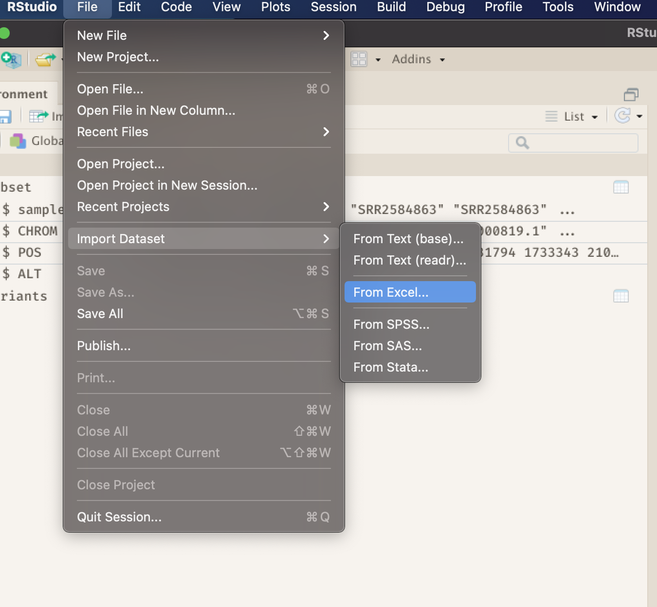
Next, under File/Url: click the Browse button and navigate to the Ecoli_metadata.xlsx file located at data/.
You should now see a preview of the data to be imported:
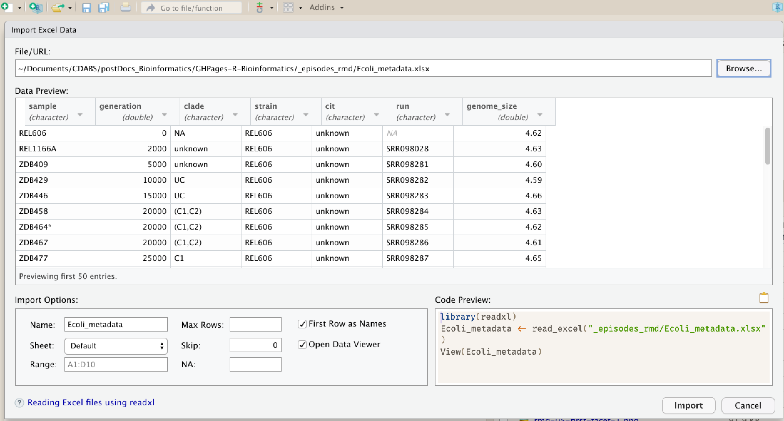
Notice that you have the option to change the data type of each variable by clicking arrow (drop-down menu) next to each column title. Under Import Options you may also rename the data, choose a different sheet to import, and choose how you will handle headers and skipped rows. Under Code Preview you can see the code that will be used to import this file. We could have written this code and imported the Excel file without the RStudio import function, but now you can choose your preference.
In this exercise, we will leave the title of the data frame as Ecoli_metadata, and there are no other options we need to adjust. Click the Import button to import the data.
Finally, let’s check the first few lines of the Ecoli_metadata data
frame:
head(Ecoli_metadata)
# A tibble: 6 × 7
  sample   generation clade   strain cit     run       genome_size
  <chr>         <dbl> <chr>   <chr>  <chr>   <chr>           <dbl>
1 REL606            0 NA      REL606 unknown <NA>             4.62
2 REL1166A       2000 unknown REL606 unknown SRR098028        4.63
3 ZDB409         5000 unknown REL606 unknown SRR098281        4.6
4 ZDB429        10000 UC      REL606 unknown SRR098282        4.59
5 ZDB446        15000 UC      REL606 unknown SRR098283        4.66
6 ZDB458        20000 (C1,C2) REL606 unknown SRR098284        4.63
The type of this object is ‘tibble’, a type of data
frame we will talk more about in the ‘dplyr’ section. If you needed
a true R data frame you could coerce with as.data.frame().
Exercise: Putting it all together - data frames
Using the
Ecoli_metadatadata frame created above, answer the following questionsA) What are the dimensions (# rows, # columns) of the data frame?
B) What are categories are there in the
citcolumn? hint: treat column as factorC) How many of each of the
citcategories are there?D) What is the genome size for the 7th observation in this data set?
E) What is the median value of the variable
genome_sizeF) Rename the column
sampletosample_idG) Create a new column (name genome_size_bp) and set it equal to the genome_size multiplied by 1,000,000
H) Save the edited Ecoli_metadata data frame as “exercise_solution.csv” in your current working directory.
Solution
A)
dim(Ecoli_metadata)[1] 30 7B)
levels(as.factor(Ecoli_metadata$cit))[1] "minus" "plus" "unknown"C)
table(as.factor(Ecoli_metadata$cit))minus plus unknown 9 9 12D)
Ecoli_metadata[7,7]# A tibble: 1 × 1 genome_size <dbl> 1 4.62E)
median(Ecoli_metadata$genome_size)[1] 4.625F)
colnames(Ecoli_metadata)[colnames(Ecoli_metadata) == "sample"] <- "sample_id"[1] "sample_id" "generation" "clade" "strain" "cit" [6] "run"G)
Ecoli_metadata$genome_size_bp <- Ecoli_metadata$genome_size * 1000000# A tibble: 6 × 8 sample_id generation clade strain cit run genome_size genome_size_bp <chr> <dbl> <chr> <chr> <chr> <chr> <dbl> <dbl> 1 REL606 0 NA REL606 unknown <NA> 4.62 4620000 2 REL1166A 2000 unknown REL606 unknown SRR098028 4.63 4630000 3 ZDB409 5000 unknown REL606 unknown SRR098281 4.6 4600000 4 ZDB429 10000 UC REL606 unknown SRR098282 4.59 4590000 5 ZDB446 15000 UC REL606 unknown SRR098283 4.66 4660000 6 ZDB458 20000 (C1,C2) REL606 unknown SRR098284 4.63 4630000H)
write.csv(Ecoli_metadata, file = "exercise_solution.csv")
Key Points
It is easy to import data into R from tabular formats including Excel. However, you still need to check that R has imported and interpreted your data correctly
There are best practices for organizing your data (keeping it tidy) and R is great for this
Base R has many useful functions for manipulating your data, but all of R’s capabilities are greatly enhanced by software packages developed by the community
Aggregating and Analyzing Data with dplyr
Overview
Teaching: 40 min
Exercises: 15 minQuestions
How can I manipulate data frames without repeating myself?
Objectives
Describe what the
dplyrpackage in R is used for.Apply common
dplyrfunctions to manipulate data in R.Employ the ‘pipe’ operator to link together a sequence of functions.
Employ the ‘mutate’ function to apply other chosen functions to existing columns and create new columns of data.
Employ the ‘split-apply-combine’ concept to split the data into groups, apply analysis to each group, and combine the results.
Bracket subsetting is handy, but it can be cumbersome and difficult to read, especially for complicated operations.
Luckily, the dplyr
package provides a number of very useful functions for manipulating data frames
in a way that will reduce repetition, reduce the probability of making
errors, and probably even save you some typing. As an added bonus, you might
even find the dplyr grammar easier to read.
Here we’re going to cover 6 of the most commonly used functions as well as using
pipes (%>%) to combine them.
glimpse()select()filter()group_by()summarize()mutate()
Packages in R are sets of additional functions that let you do more
stuff in R. The functions we’ve been using, like str(), come built into R;
packages give you access to more functions. You need to install a package and
then load it to be able to use it.
install.packages("dplyr") ## install
You might get asked to choose a CRAN mirror – this is asking you to choose a site to download the package from. The choice doesn’t matter too much; I’d recommend choosing the RStudio mirror.
library("dplyr") ## load
You only need to install a package once per computer, but you need to load it every time you open a new R session and want to use that package.
What is dplyr?
The package dplyr is a fairly new (2014) package that tries to provide easy
tools for the most common data manipulation tasks. This package is also included in the tidyverse package, which is a collection of eight different packages (dplyr, ggplot2, tibble, tidyr, readr, purrr, stringr, and forcats). It is built to work directly
with data frames. The thinking behind it was largely inspired by the package
plyr which has been in use for some time but suffered from being slow in some
cases. dplyr addresses this by porting much of the computation to C++. An
additional feature is the ability to work with data stored directly in an
external database. The benefits of doing this are that the data can be managed
natively in a relational database, queries can be conducted on that database,
and only the results of the query returned.
This addresses a common problem with R in that all operations are conducted in memory and thus the amount of data you can work with is limited by available memory. The database connections essentially remove that limitation in that you can have a database that is over 100s of GB, conduct queries on it directly and pull back just what you need for analysis in R.
Taking a quick look at data frames
Similar to str(), which comes built into R, glimpse() is a dplyr function that (as the name suggests) gives a glimpse of the data frame.
Rows: 801
Columns: 29
$ sample_id     <chr> "SRR2584863", "SRR2584863", "SRR2584863", "SRR2584863", …
$ CHROM         <chr> "CP000819.1", "CP000819.1", "CP000819.1", "CP000819.1", …
$ POS           <dbl> 9972, 263235, 281923, 433359, 473901, 648692, 1331794, 1…
$ ID            <lgl> NA, NA, NA, NA, NA, NA, NA, NA, NA, NA, NA, NA, NA, NA, …
$ REF           <chr> "T", "G", "G", "CTTTTTTT", "CCGC", "C", "C", "G", "ACAGC…
$ ALT           <chr> "G", "T", "T", "CTTTTTTTT", "CCGCGC", "T", "A", "A", "AC…
$ QUAL          <dbl> 91.0000, 85.0000, 217.0000, 64.0000, 228.0000, 210.0000,…
$ FILTER        <lgl> NA, NA, NA, NA, NA, NA, NA, NA, NA, NA, NA, NA, NA, NA, …
$ INDEL         <lgl> FALSE, FALSE, FALSE, TRUE, TRUE, FALSE, FALSE, FALSE, TR…
$ IDV           <dbl> NA, NA, NA, 12, 9, NA, NA, NA, 2, 7, NA, NA, NA, NA, NA,…
$ IMF           <dbl> NA, NA, NA, 1.000000, 0.900000, NA, NA, NA, 0.666667, 1.…
$ DP            <dbl> 4, 6, 10, 12, 10, 10, 8, 11, 3, 7, 9, 20, 12, 19, 15, 10…
$ VDB           <dbl> 0.0257451, 0.0961330, 0.7740830, 0.4777040, 0.6595050, 0…
$ RPB           <dbl> NA, 1.000000, NA, NA, NA, NA, NA, NA, NA, NA, 0.900802, …
$ MQB           <dbl> NA, 1.0000000, NA, NA, NA, NA, NA, NA, NA, NA, 0.1501340…
$ BQB           <dbl> NA, 1.000000, NA, NA, NA, NA, NA, NA, NA, NA, 0.750668, …
$ MQSB          <dbl> NA, NA, 0.974597, 1.000000, 0.916482, 0.916482, 0.900802…
$ SGB           <dbl> -0.556411, -0.590765, -0.662043, -0.676189, -0.662043, -…
$ MQ0F          <dbl> 0.000000, 0.166667, 0.000000, 0.000000, 0.000000, 0.0000…
$ ICB           <lgl> NA, NA, NA, NA, NA, NA, NA, NA, NA, NA, NA, NA, NA, NA, …
$ HOB           <lgl> NA, NA, NA, NA, NA, NA, NA, NA, NA, NA, NA, NA, NA, NA, …
$ AC            <dbl> 1, 1, 1, 1, 1, 1, 1, 1, 1, 1, 1, 1, 1, 1, 1, 1, 1, 1, 1,…
$ AN            <dbl> 1, 1, 1, 1, 1, 1, 1, 1, 1, 1, 1, 1, 1, 1, 1, 1, 1, 1, 1,…
$ DP4           <chr> "0,0,0,4", "0,1,0,5", "0,0,4,5", "0,1,3,8", "1,0,2,7", "…
$ MQ            <dbl> 60, 33, 60, 60, 60, 60, 60, 60, 60, 60, 25, 60, 10, 60, …
$ Indiv         <chr> "/home/dcuser/dc_workshop/results/bam/SRR2584863.aligned…
$ gt_PL         <dbl> 1210, 1120, 2470, 910, 2550, 2400, 2080, 2550, 11128, 19…
$ gt_GT         <dbl> 1, 1, 1, 1, 1, 1, 1, 1, 1, 1, 1, 1, 1, 1, 1, 1, 1, 1, 1,…
$ gt_GT_alleles <chr> "G", "T", "T", "CTTTTTTTT", "CCGCGC", "T", "A", "A", "AC…
In the above output, we can already gather some information about variants, such as the number of rows and columns, column names, type of vector in the columns, and the first few entries of each column. Although what we see is similar to outputs of str(), this method gives a cleaner visual output.
Selecting columns and filtering rows
To select columns of a data frame, use select(). The first argument to this function is the data frame (variants), and the subsequent arguments are the columns to keep.
select(variants, sample_id, REF, ALT, DP)
# A tibble: 6 × 4
  sample_id  REF      ALT          DP
  <chr>      <chr>    <chr>     <dbl>
1 SRR2584863 T        G             4
2 SRR2584863 G        T             6
3 SRR2584863 G        T            10
4 SRR2584863 CTTTTTTT CTTTTTTTT    12
5 SRR2584863 CCGC     CCGCGC       10
6 SRR2584863 C        T            10
To select all columns except certain ones, put a “-“ in front of the variable to exclude it.
select(variants, -CHROM)
# A tibble: 6 × 28
  sample_id     POS ID    REF   ALT    QUAL FILTER INDEL   IDV   IMF    DP    VDB
  <chr>       <dbl> <lgl> <chr> <chr> <dbl> <lgl>  <lgl> <dbl> <dbl> <dbl>  <dbl>
1 SRR2584863   9972 NA    T     G        91 NA     FALSE    NA  NA       4 0.0257
2 SRR2584863 263235 NA    G     T        85 NA     FALSE    NA  NA       6 0.0961
3 SRR2584863 281923 NA    G     T       217 NA     FALSE    NA  NA      10 0.774
4 SRR2584863 433359 NA    CTTT… CTTT…    64 NA     TRUE     12   1      12 0.478
5 SRR2584863 473901 NA    CCGC  CCGC…   228 NA     TRUE      9   0.9    10 0.660
6 SRR2584863 648692 NA    C     T       210 NA     FALSE    NA  NA      10 0.268
# … with 16 more variables: RPB <dbl>, MQB <dbl>, BQB <dbl>, MQSB <dbl>,
#   SGB <dbl>, MQ0F <dbl>, ICB <lgl>, HOB <lgl>, AC <dbl>, AN <dbl>, DP4 <chr>,
#   MQ <dbl>, Indiv <chr>, gt_PL <dbl>, gt_GT <dbl>, gt_GT_alleles <chr>
To choose rows, use filter():
filter(variants, sample_id == "SRR2584863")
# A tibble: 6 × 29
  sample_id  CHROM    POS ID    REF   ALT    QUAL FILTER INDEL   IDV   IMF    DP
  <chr>      <chr>  <dbl> <lgl> <chr> <chr> <dbl> <lgl>  <lgl> <dbl> <dbl> <dbl>
1 SRR2584863 CP00…   9972 NA    T     G        91 NA     FALSE    NA  NA       4
2 SRR2584863 CP00… 263235 NA    G     T        85 NA     FALSE    NA  NA       6
3 SRR2584863 CP00… 281923 NA    G     T       217 NA     FALSE    NA  NA      10
4 SRR2584863 CP00… 433359 NA    CTTT… CTTT…    64 NA     TRUE     12   1      12
5 SRR2584863 CP00… 473901 NA    CCGC  CCGC…   228 NA     TRUE      9   0.9    10
6 SRR2584863 CP00… 648692 NA    C     T       210 NA     FALSE    NA  NA      10
# … with 17 more variables: VDB <dbl>, RPB <dbl>, MQB <dbl>, BQB <dbl>,
#   MQSB <dbl>, SGB <dbl>, MQ0F <dbl>, ICB <lgl>, HOB <lgl>, AC <dbl>,
#   AN <dbl>, DP4 <chr>, MQ <dbl>, Indiv <chr>, gt_PL <dbl>, gt_GT <dbl>,
#   gt_GT_alleles <chr>
Note that this is equivalent to the base R code below, but is easier to read!
variants[variants$sample_id == "SRR2584863",]
Pipes
But what if you wanted to select and filter? We can do this with pipes. Pipes, are a fairly recent addition to R. Pipes let you
take the output of one function and send it directly to the next, which is
useful when you need to many things to the same data set. It was
possible to do this before pipes were added to R, but it was
much messier and more difficult. Pipes in R look like
%>% and are made available via the magrittr package, which is installed as
part of dplyr. If you use RStudio, you can type the pipe with
Ctrl + Shift + M if you’re using a PC,
or Cmd + Shift + M if you’re using a Mac.
variants %>%
  filter(sample_id == "SRR2584863") %>%
  select(REF, ALT, DP) %>%
  head()
# A tibble: 6 × 3
  REF      ALT          DP
  <chr>    <chr>     <dbl>
1 T        G             4
2 G        T             6
3 G        T            10
4 CTTTTTTT CTTTTTTTT    12
5 CCGC     CCGCGC       10
6 C        T            10
In the above code, we use the pipe to send the variants dataset first through
filter(), to keep rows where sample_id matches a particular sample, and then through select() to
keep only the REF, ALT, and DP columns. Since %>% takes
the object on its left and passes it as the first argument to the function on
its right, we don’t need to explicitly include the data frame as an argument
to the filter() and select() functions any more. We then pipe the results
to the head() function so that we only see the first six rows of data.
Some may find it helpful to read the pipe like the word “then”. For instance,
in the above example, we took the data frame variants, then we filtered
for rows where sample_id was SRR2584863, then we selected the REF, ALT, and DP columns, then we showed only the first six rows.
The dplyr functions by themselves are somewhat simple,
but by combining them into linear workflows with the pipe, we can accomplish
more complex manipulations of data frames.
If we want to create a new object with this smaller version of the data we can do so by assigning it a new name:
SRR2584863_variants <- variants %>%
  filter(sample_id == "SRR2584863") %>%
  select(REF, ALT, DP)
This new object includes all of the data from this sample. Let’s look at just the first six rows to confirm it’s what we want:
SRR2584863_variants %>% head()
# A tibble: 6 × 3
  REF      ALT          DP
  <chr>    <chr>     <dbl>
1 T        G             4
2 G        T             6
3 G        T            10
4 CTTTTTTT CTTTTTTTT    12
5 CCGC     CCGCGC       10
6 C        T            10
Similar to head() and tail() functions, we can also look at the first or last six rows using tidyverse function slice(). The differences between these two functions are minimal. The advantage of slice() is that you are not bound by the first or last Nth rows, and specific rows can be viewed:
SRR2584863_variants %>% slice(1:6)
# A tibble: 6 × 3
  REF      ALT          DP
  <chr>    <chr>     <dbl>
1 T        G             4
2 G        T             6
3 G        T            10
4 CTTTTTTT CTTTTTTTT    12
5 CCGC     CCGCGC       10
6 C        T            10
SRR2584863_variants %>% slice(10:15)
# A tibble: 6 × 3
  REF   ALT      DP
  <chr> <chr> <dbl>
1 AT    ATT       7
2 A     C         9
3 A     C        20
4 G     T        12
5 A     T        19
6 G     A        15
Exercise: Pipe and filter
Starting with the
variantsdata frame, use pipes to subset the data to include only observations from SRR2584863 sample, where the filtered depth (DP) is at least 10. Retain only the columnsREF,ALT, andPOS.Solution
 variants %>%
 filter(sample_id == "SRR2584863" & DP >= 10) %>%
 select(REF, ALT, POS)
# A tibble: 16 × 3 REF ALT POS <chr> <chr> <dbl> 1 G T 281923 2 CTTTTTTT CTTTTTTTT 433359 3 CCGC CCGCGC 473901 4 C T 648692 5 G A 1733343 6 A C 2446984 7 G T 2618472 8 A T 2665639 9 G A 2999330 10 A C 3339313 11 C A 3401754 12 A C 3488669 13 G T 3909807 14 A G 4100183 15 A C 4201958 16 TGG T 4431393
Mutate
Frequently you’ll want to create new columns based on the values in existing
columns, for example to do unit conversions or find the ratio of values in two
columns. For this we’ll use the dplyr function mutate().
We have a column titled “QUAL”. This is a Phred-scaled confidence score that a polymorphism exists at this position given the sequencing data. Lower QUAL scores indicate low probability of a polymorphism existing at that site. We can convert the confidence value QUAL to a probability value according to the formula:
Probability = 1- 10 ^ -(QUAL/10)
Let’s add a column (POLPROB) to our variants data frame that shows
the probability of a polymorphism at that site given the data. We’ll show
only the first six rows of data.
variants %>%
  mutate(POLPROB = 1 - (10 ^ -(QUAL/10))) %>%
  head()
# A tibble: 6 × 30
  sample_id  CHROM    POS ID    REF   ALT    QUAL FILTER INDEL   IDV   IMF    DP
  <chr>      <chr>  <dbl> <lgl> <chr> <chr> <dbl> <lgl>  <lgl> <dbl> <dbl> <dbl>
1 SRR2584863 CP00…   9972 NA    T     G        91 NA     FALSE    NA  NA       4
2 SRR2584863 CP00… 263235 NA    G     T        85 NA     FALSE    NA  NA       6
3 SRR2584863 CP00… 281923 NA    G     T       217 NA     FALSE    NA  NA      10
4 SRR2584863 CP00… 433359 NA    CTTT… CTTT…    64 NA     TRUE     12   1      12
5 SRR2584863 CP00… 473901 NA    CCGC  CCGC…   228 NA     TRUE      9   0.9    10
6 SRR2584863 CP00… 648692 NA    C     T       210 NA     FALSE    NA  NA      10
# … with 18 more variables: VDB <dbl>, RPB <dbl>, MQB <dbl>, BQB <dbl>,
#   MQSB <dbl>, SGB <dbl>, MQ0F <dbl>, ICB <lgl>, HOB <lgl>, AC <dbl>,
#   AN <dbl>, DP4 <chr>, MQ <dbl>, Indiv <chr>, gt_PL <dbl>, gt_GT <dbl>,
#   gt_GT_alleles <chr>, POLPROB <dbl>
Exercise
There are a lot of columns in our dataset, so let’s just look at the
sample_id,POS,QUAL, andPOLPROBcolumns for now. Add a line to the above code to only show those columns.Solution
variants %>%
 mutate(POLPROB = 1 - 10 ^ -(QUAL/10)) %>%
 select(sample_id, POS, QUAL, POLPROB) %>%
 head
# A tibble: 6 × 4 sample_id POS QUAL POLPROB <chr> <dbl> <dbl> <dbl> 1 SRR2584863 9972 91 1.00 2 SRR2584863 263235 85 1.00 3 SRR2584863 281923 217 1 4 SRR2584863 433359 64 1.00 5 SRR2584863 473901 228 1 6 SRR2584863 648692 210 1
Split-apply-combine data analysis and the summarize() function
Many data analysis tasks can be approached using the “split-apply-combine”
paradigm: split the data into groups, apply some analysis to each group, and
then combine the results. dplyr makes this very easy through the use of the
group_by() function, which splits the data into groups. When the data is
grouped in this way summarize() can be used to collapse each group into
a single-row summary. summarize() does this by applying an aggregating
or summary function to each group. For example, if we wanted to group
by sample_id and find the number of rows of data for each
sample, we would do:
variants %>%
  group_by(sample_id) %>%
  summarize(n())
# A tibble: 3 × 2
  sample_id  `n()`
  <chr>      <int>
1 SRR2584863    25
2 SRR2584866   766
3 SRR2589044    10
It can be a bit tricky at first, but we can imagine physically splitting the data frame by groups and applying a certain function to summarize the data.
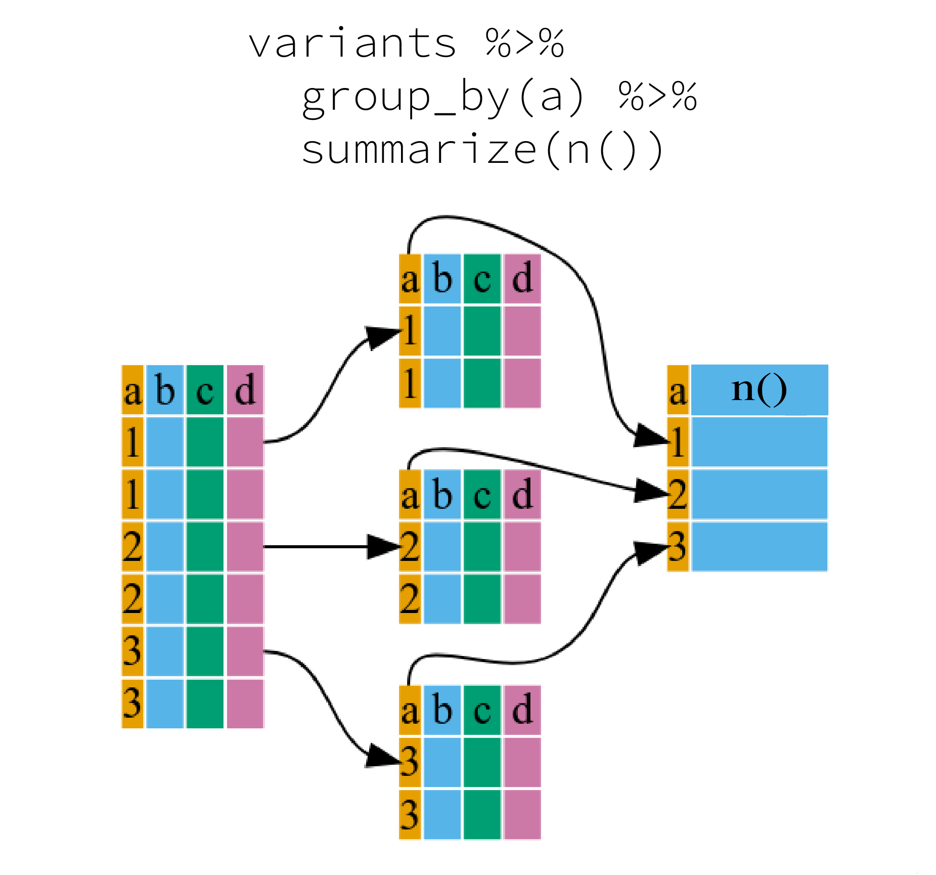
^[The figure was adapted from the Software Carpentry lesson, R for Reproducible Scientific Analysis]
Here the summary function used was n() to find the count for each
group. Since this is a quite a common operation, there is a simpler method
called tally():
variants %>%
  group_by(sample_id) %>%
  tally()
# A tibble: 3 × 2
  sample_id      n
  <chr>      <int>
1 SRR2584863    25
2 SRR2584866   766
3 SRR2589044    10
To show that there are many ways to acheive the same results, there is another way to appraoch this, which bypasses group_by() using the function count():
variants %>%
  count(sample_id)
# A tibble: 3 × 2
  sample_id      n
  <chr>      <int>
1 SRR2584863    25
2 SRR2584866   766
3 SRR2589044    10
We can also apply many other functions to individual columns to get other
summary statistics. For example,we can use built-in functions like mean(),
median(), min(), and max(). These are called “built-in functions” because
they come with R and don’t require that you install any additional packages.
By default, all R functions operating on vectors that contains missing data will return NA.
It’s a way to make sure that users know they have missing data, and make a
conscious decision on how to deal with it. When dealing with simple statistics
like the mean, the easiest way to ignore NA (the missing data) is
to use na.rm = TRUE (rm stands for remove).
So to view the highest filtered depth (DP) for each sample:
variants %>%
  group_by(sample_id) %>%
  summarize(max(DP))
# A tibble: 3 × 2
  sample_id  `max(DP)`
  <chr>          <dbl>
1 SRR2584863        20
2 SRR2584866        79
3 SRR2589044        16
Much of this lesson was copied or adapted from Jeff Hollister’s materials
Key Points
Use the
dplyrpackage to manipulate data frames.Use
glimpse()to quickly look at your data frame.Use
select()to choose variables from a data frame.Use
filter()to choose data based on values.Use
mutate()to create new variables.Use
group_by()andsummarize()to work with subsets of data.
Data Visualization with ggplot2
Overview
Teaching: 60 min
Exercises: 30 minQuestions
How can I create publication-quality graphics in R?
How do I save a ggplot2 object I just created?
Objectives
To be able to use ggplot2 to generate publication quality graphics.
Describe the role of data, aesthetics, and geoms in ggplot functions.
Choose the correct aesthetics and alter the geom parameters for a scatter plot, histogram, or box plot.
Layer multiple geometries in a single plot.
Customize plot scales, titles, subtitles, themes, fonts, layout, and orientation.
Apply a facet to a plot.
Apply additional ggplot2-compatible plotting libraries.
Save a ggplot to a file.
List several resources for getting help with ggplot.
List several resources for creating informative scientific plots.
We start by loading the package ggplot2.
library(ggplot2)
Plotting with ggplot2
ggplot2 is a plotting package that makes it simple to create complex plots
from data in a data frame. It provides a more programmatic interface for
specifying what variables to plot, how they are displayed, and general visual
properties. Therefore, we only need minimal changes if the underlying data change
or if we decide to change from a bar plot to a scatter plot. This helps in creating
publication quality plots with minimal amounts of adjustments and tweaking.
ggplot2 functions like data in the ‘long’ format, i.e., a column for every dimension,
and a row for every observation. Well-structured data will save you lots of time
when making figures with ggplot2
ggplot graphics are built step by step by adding new elements. Adding layers in this fashion allows for extensive flexibility and customization of plots.
To build a ggplot, we will use the following basic template that can be used for different types of plots:
ggplot(data = <DATA>, mapping = aes(<MAPPINGS>)) + <GEOM_FUNCTION>()
- use the
ggplot()function and bind the plot to a specific data frame using thedataargument
ggplot(data = variants)
- define a mapping (using the aesthetic (
aes) function), by selecting the variables to be plotted and specifying how to present them in the graph, e.g. as x/y positions or characteristics such as size, shape, color, etc.
ggplot(data = variants, aes(x = POS, y = DP))
-
add ‘geoms’ – graphical representations of the data in the plot (points, lines, bars).
ggplot2offers many different geoms; we will use some common ones today, including:* `geom_point()` for scatter plots, dot plots, etc. * `geom_boxplot()` for, well, boxplots! * `geom_line()` for trend lines, time series, etc.
To add a geom to the plot use the + operator. Because we have two continuous variables,
let’s use geom_point() first:
ggplot(data = variants, aes(x = POS, y = DP)) +
  geom_point()

The + in the ggplot2 package is particularly useful because it allows you
to modify existing ggplot objects. This means you can easily set up plot
templates and conveniently explore different types of plots, so the above
plot can also be generated with code like this:
# Assign plot to a variable
coverage_plot <- ggplot(data = variants, aes(x = POS, y = DP))

# Draw the plot
coverage_plot +
    geom_point()
Notes
- Anything you put in the
ggplot()function can be seen by any geom layers that you add (i.e., these are universal plot settings). This includes the x- and y-axis mapping you set up inaes(). - You can also specify mappings for a given geom independently of the
mappings defined globally in the
ggplot()function. - The
+sign used to add new layers must be placed at the end of the line containing the previous layer. If, instead, the+sign is added at the beginning of the line containing the new layer,ggplot2will not add the new layer and will return an error message.
# This is the correct syntax for adding layers
coverage_plot +
  geom_point()

# This will not add the new layer and will return an error message
coverage_plot
  + geom_point()
Building your plots iteratively
Building plots with ggplot2 is typically an iterative process. We start by
defining the dataset we’ll use, lay out the axes, and choose a geom:
ggplot(data = variants, aes(x = POS, y = DP)) +
  geom_point()

Then, we start modifying this plot to extract more information from it. For
instance, we can add transparency (alpha) to avoid overplotting:
ggplot(data = variants, aes(x = POS, y = DP)) +
    geom_point(alpha = 0.5)

We can also add colors for all the points:
ggplot(data = variants, aes(x = POS, y = DP)) +
  geom_point(alpha = 0.5, color = "blue")

Or to color each species in the plot differently, you could use a vector as an input to the argument color. ggplot2 will provide a different color corresponding to different values in the vector. Here is an example where we color with sample_id:
ggplot(data = variants, aes(x = POS, y = DP, color = sample_id)) +
  geom_point(alpha = 0.5)

Notice that we can change the geom layer and colors will be still determined by sample_id
ggplot(data = variants, aes(x = POS, y = DP, color = sample_id)) +
  geom_jitter(alpha = 0.5)

To make our plot more readable, we can add axis labels:
ggplot(data = variants, aes(x = POS, y = DP, color = sample_id)) +
  geom_jitter(alpha = 0.5) +
  labs(x = "Base Pair Position",
       y = "Read Depth (DP)")

Challenge
Use what you just learned to create a scatter plot of mapping quality (
MQ) over position (POS) with the samples showing in different colors. Make sure to give your plot relevant axis labels.Solution
 ggplot(data = variants, aes(x = POS, y = MQ, color = sample_id)) +
  geom_point() +
  labs(x = "Base Pair Position",
       y = "Mapping Quality (MQ)")

Faceting
ggplot2 has a special technique called faceting that allows the user to split one
plot into multiple plots based on a factor included in the dataset. We will use it to split our
mapping quality plot into three panels, one for each sample.
ggplot(data = variants, aes(x = POS, y = MQ, color = sample_id)) +
 geom_point() +
 labs(x = "Base Pair Position",
      y = "Mapping Quality (MQ)") +
 facet_grid(. ~ sample_id)

This looks ok, but it would be easier to read if the plot facets were stacked vertically rather
than horizontally. The facet_grid
geometry allows you to explicitly specify how you want your plots to be
arranged via formula notation (rows ~ columns; a . can be used as
a placeholder that indicates only one row or column).
ggplot(data = variants, aes(x = POS, y = MQ, color = sample_id)) +
 geom_point() +
 labs(x = "Base Pair Position",
      y = "Mapping Quality (MQ)") +
 facet_grid(sample_id ~ .)

Usually plots with white background look more readable when printed. We can set
the background to white using the function theme_bw(). Additionally, you can remove
the grid:
ggplot(data = variants, aes(x = POS, y = MQ, color = sample_id)) +
  geom_point() +
  labs(x = "Base Pair Position",
       y = "Mapping Quality (MQ)") +
  facet_grid(sample_id ~ .) +
  theme_bw() +
  theme(panel.grid = element_blank())

Challenge
Use what you just learned to create a scatter plot of PHRED scaled quality (
QUAL) over position (POS) with the samples showing in different colors. Make sure to give your plot relevant axis labels.Solution
 ggplot(data = variants, aes(x = POS, y = QUAL, color = sample_id)) +
  geom_point() +
  labs(x = "Base Pair Position",
       y = "PHRED-sacled Quality (QUAL)") +
  facet_grid(sample_id ~ .)

Exporting the plot
The ggsave() function allows you to export a plot created with ggplot. You can specify the dimension and resolution of your plot by adjusting the appropriate arguments (width, height and dpi) to create high quality graphics for publication. In order to save the plot from above, we first assign it to a variable facet-plot-white-bg, then tell ggsave to save that plot in png format to a directory called results. (Make sure you have a results/ folder in your working directory.)
facet-plot-white-bg <- ggplot(data = variants, aes(x = POS, y = MQ, color = sample_id)) +
  geom_point() +
  labs(x = "Base Pair Position",
       y = "Mapping Quality (MQ)") +
  facet_grid(sample_id ~ .) +
  theme_bw() +
  theme(panel.grid = element_blank())

ggsave(filename = "results/facet-plot-white-bg.png", plot = facet-plot-white-bg, width = 12, height = 10, dpi = 300, units = "cm")
There are two nice things about ggsave. First, it defaults to the last plot, so if you omit the plot argument it will automatically save the last plot you created with ggplot. Secondly, it tries to determine the format you want to save your plot in from the file extension you provide for the filename (for example .png or .pdf). If you need to, you can specify the format explicitly in the device argument.
Barplots
We can create barplots using the geom_bar geom. Let’s make a barplot showing
the number of variants for each sample that are indels.
ggplot(data = variants, aes(x = INDEL, fill = sample_id)) +
  geom_bar() +
  facet_grid(sample_id ~ .)

Challenge
Since we already have the sample_id labels on the individual plot facets, we don’t need the legend. Use the help file for
geom_barand any other online resources you want to use to remove the legend from the plot.Solution
ggplot(data = variants, aes(x = INDEL, color = sample_id)) +
   geom_bar(show.legend = F) +
   facet_grid(sample_id ~ .)

ggplot2 themes
In addition to theme_bw(), which changes the plot background to white, ggplot2
comes with several other themes which can be useful to quickly change the look
of your visualization. The complete list of themes is available
at https://ggplot2.tidyverse.org/reference/ggtheme.html. theme_minimal() and
theme_light() are popular, and theme_void() can be useful as a starting
point to create a new hand-crafted theme.
The
ggthemes package
provides a wide variety of options (including an Excel 2003 theme).
The ggplot2 extensions website provides a list
of packages that extend the capabilities of ggplot2, including additional
themes.
Challenge
With all of this information in hand, please take another five minutes to either improve one of the plots generated in this exercise or create a beautiful graph of your own. Use the RStudio
ggplot2cheat sheet for inspiration. Here are some ideas:
- See if you can change the size or shape of the plotting symbol.
- Can you find a way to change the name of the legend? What about its labels?
- Try using a different color palette (see http://www.cookbook-r.com/Graphs/Colors_(ggplot2)/).
Key Points
Use
ggplot2to create plots.Think about graphics in layers: aesthetics, geometry, statistics, scale transformation, and grouping.
Producing Reports With R Markdown and knitr
Overview
Teaching: 60 min
Exercises: 15 minQuestions
How can I integrate software and reports?
Objectives
Value of reproducible reports
Basics of Markdown
R code chunks
Chunk options
Inline R code
Other output formats
Reproducible Reports with R Markdown
It doesn’t matter how great your analysis is unless you can explain it to others and provide your analysis in a way that is reproducibly by others: you need to communicate your results.
Many new users begin by first writing a single R script containing all of their work, and then share the analysis by emailing the script and various graphs as attachments. But this can be cumbersome, requiring a lengthy discussion to explain which attachment was which result.
Writing formal reports with Word can simplify this process by incorporating both the analysis report and output graphs into a single document. But tweaking formatting to make figures look correct and fixing obnoxious page breaks can be tedious and lead to a lengthy “whack-a-mole” game of fixing new mistakes resulting from a single formatting change.
What is R Markdown

R Markdown provides an authoring framework for data science. You can use a single R Markdown file to both
-
save and execute code, and
-
generate high quality reports that can be shared with an audience.
R Markdown was designed for easier reproducibility, since both the computing code and narratives are in the same document, and results are automatically generated from the source code. R Markdown supports dozens of static and dynamic/interactive output formats like word, pdf, powerpoint and more!
To use Rmarkdown you need the rmarkdown package, but you don’t need to explicitly install it or load it, as RStudio automatically does both when needed.
R Markdown Related Packages

In addition to the amazing reports and even slide decks that you can produce with Rmarkdown one of the other amazing features is that it can also be used to create your own website using the package blogdown and author books using the bookdown package. These two abilities truly extend the reach of your work essentially making it available to anyone with a web browser and internet connection.
bookdown is an R package that allows you to write books and long-form reports with multiple Rmd files. After this package was published, a large number of books have emerged. You can find a subset of them at (https://bookdown.org). Some of these books have been printed, and some only have free online versions.
There have also been students who wrote their dissertations/theses with bookdown, such as Ed Berry: (https://eddjberry.netlify.com/post/writing-your-thesis-with-bookdown/). Chester Ismay has even provided an R package thesisdown (https://github.com/ismayc/thesisdown) that can render a thesis in various formats.
The blogdown package can be used to build general-purpose websites (including blogs and personal websites) based on R Markdown. You may find tons of examples at (https://github.com/rbind) or by searching on Twitter: (https://twitter.com/search?q=blogdown).
How does R Markdown work
Lets take a look under the hood at R Markdown. The best way to get a sense of whats going on is to create a R Markdown file using RStudio.
Creating an R Markdown file
Within RStudio, click File → New File → R Markdown and you’ll get a dialog box like this:

You can stick with the default (HTML output), but give it a title.
As a result RStudio generates this:

R Markdown Basic Components
What we see is an R Markdown file, a plain text file that has the extension .Rmd: It contains three important types of content:
- An (optional) YAML header surrounded by
---s. - Chunks of R code surrounded by
```. - Text mixed with simple text formatting like
# headingand_italics_.
YAML Header
The initial chunk of text (header) contains instructions for R to specify what kind of document will be created, and the options chosen. You can use the header to give your document a title, author, date, and tell it what type of output you want to produce. In this case, we’re creating an html document. The syntax for the metadata is YAML (YAML Ain’t Markup Language, (https://en.wikipedia.org/wiki/YAML)), so sometimes it is also called the YAML metadata or the YAML frontmatter. Before it bites you hard, we want to warn you in advance that indentation matters in YAML, so do not forget to indent the sub-fields of a top field properly.
---
title: "post-docs-bioinformatics-Rmd-Practice"
author: "JP Courneya"
date: "7/21/2021"
output: html_document
---
Body of the document
The body of the document follows the metadata. The syntax for text (also known as prose or narratives) is Markdown, a lightweight set of conventions for formatting plain text files. Markdown is designed to be easy to read and easy to write. There are also two types of computer code, code chunks and inline R code. We will look at each of these in more detail in subsequent sections.
You will notice in the .Rmd interface the code and output are interleaved. You can run each code chunk by clicking the Run icon (it looks like a play button at the top of the chunk), or by pressing Cmd/Ctrl+Shift+Enter. RStudio executes the code and displays the results inline with the code:

To generate a report from the file, run the render command:
library(rmarkdown)
render("post-docs-bioinformatics-rmd-practice.Rmd")
Better still, use the:  button in the RStudio IDE to render the file and preview the output with a single click. You will notice your first time “knitting” the document you are prompted to save the file, save it with a meaningful name.

R Markdown generates a new file that contains selected text, code, and results from the .Rmd file.
How things get compiled

When you run render, or press the Knit button, R Markdown feeds the .Rmd file to knitr, which executes all of the code chunks and creates a new markdown (.md) document which includes the code and its output.
The markdown file generated by knitr is then processed by pandoc which is responsible for creating the finished format.
This may sound complicated, but R Markdown makes it extremely simple by encapsulating all of the above processing into a single render function or Knit button.
Markdown
Markdown is a system for writing web pages by marking up the text much as you would in an email rather than writing html code. The marked-up text gets converted to html, replacing the marks with the proper html code.
For now, let’s delete all of the stuff that’s in the .Rmd file and write a bit of markdown.
You make things bold using two asterisks, like this: **bold**, and you make things italics by using underscores, like this: _italics_.
You can make a bulleted list by writing a list with hyphens or asterisks, like this:
* one item
* one item
* one item
    * one more item
    * one more item
    * one more item

- bold with double-asterisks
- italics with underscores
- code-type font with backticks
The output is:
- one item
- one item
- one item
- one more item
- one more item
- one more item
- bold with double-asterisks
- italics with underscores
- code-type font with backticks
You can use whatever method you prefer, but be consistent. This maintains the readability of your code.
You can make a numbered list by just using numbers. You can even use the same number over and over if you want:
1. bold with double-asterisks
1. italics with underscores
1. code-type font with backticks
This will appear as:
- bold with double-asterisks
- italics with underscores
- code-type font with backticks
You can make section headers of different sizes by initiating a line with some number of # symbols:
# Title
## Main section
### Sub-section
#### Sub-sub section
They will appear like this:

A bit more Markdown
You can make a hyperlink like this: [text to show](http://the-web-page.com).
You can include an image file like this: 
You can do subscripts (e.g., F~2~) with F~2~ and superscripts (e.g., F^2^) with F^2^.
If you know how to write equations in LaTeX, you can use $ $ and $$ $$ to insert math equations, like $E = mc^2$ and
$$y = \mu + \sum_{i=1}^p \beta_i x_i + \epsilon$$
R code chunks
The real power of Markdown comes from mixing markdown with chunks of code. This is R Markdown. When processed, the R code will be executed; if they produce figures, the figures will be inserted in the final document.
To run code inside an R Markdown document, you need to insert a chunk. There are three ways to do so:
-
The keyboard shortcut Cmd/Ctrl+Alt+I
-
The “Insert” button icon in the editor toolbar.
-
By manually typing the chunk delimiters
```{r}and```.
I’d recommend you learn the keyboard shortcut. It will save you a lot of time in the long run!
The main code chunks look like this:
```{r}
    summary(cars)
```
You should give each chunk a unique name, as they will help you to fix errors and, if any graphs are produced, the file names are based on the name of the code chunk that produced them.
Exercise: Add code chunks to your R Markdown Document:
A) Download the gapminder data from here.
- Download the file (CTRL + S, right mouse click -> “Save as”, or File -> “Save page as”)
- Make sure it’s saved under the name
gapminder-FiveYearData.csv- Save the file in the
data/folder within your project.B) Load the
ggplot2packageC) Read the gapminder data to an object named
gapminderD) Create a plot of
lifeExp ~ yearSolution
```{r download-gapminder-data, eval=TRUE}
download.file("https://raw.githubusercontent.com/resbaz/r-novice-gapminder-files/master/data/gapminder-FiveYearData.csv", destfile = >>"data/gapminder-FiveYearData.csv")
```

```{r load-ggplot2, eval=TRUE}
library("ggplot2")
```

```{r read-gapminder-data, eval=TRUE}
gapminder <- read.csv(file = "data/gapminder_data.csv", stringsAsFactors = >>TRUE)
```

```{r make-plot, eval=TRUE}
plot(lifeExp ~ year, data = gapminder)
```
Chunk Options
There are a variety of options to affect how the code chunks are treated. Here are some examples:
- Use
echo=FALSEto avoid having the code itself shown. - Use
results="hide"to avoid having any results printed. - Use
eval=FALSEto have the code shown but not evaluated. - Use
warning=FALSEandmessage=FALSEto hide any warnings or messages produced. - Use
fig.heightandfig.widthto control the size of the figures produced (in inches).
So you might write:
```{r load_libraries, echo=FALSE, message=FALSE}
library("dplyr")
library("ggplot2")
```
Often there will be particular options that you’ll want to use repeatedly; for this, you can set global chunk options, like so:
```{r global_options, echo=FALSE}
knitr::opts_chunk$set(fig.path="Figs/", message=FALSE, warning=FALSE, echo=FALSE, results="hide", fig.width=11)
```
The fig.path option defines where the figures will be saved. The / here is really important; without it, the figures would be saved in the standard place but just with names that begin with Figs.
If you have multiple R Markdown files in a common directory, you might want to use fig.path to define separate prefixes for the figure file names, like fig.path="Figs/cleaning-" and fig.path="Figs/analysis-".
You can review all of the R chunk options by navigating to the “R Markdown Cheat Sheet” under the “Cheatsheets” section of the “Help” field in the toolbar at the top of RStudio.
Inline code
There is one other way to embed R code into an R Markdown document: directly into the text, with: r.
This can be very useful if you mention properties of your data in the text.
For example, using the diamonds dataset we could report:
We have data about
r nrow(ggplot2::diamondsdiamonds.
The output would be:
We have data about 53940 diamonds.
When inserting numbers into text, format() is your friend.
It allows you to set the number of digits so you don’t print to a ridiculous degree of accuracy, and a big.mark to make numbers easier to read.
The expression:
We have data about
`r format(nrow(ggplot2::diamonds), digits = 2, big.mark = ",")`diamonds.
Would look like this:
We have data about 53,940 diamonds.
You can combine these into a helper function:
comma <- function(x) format(x, digits = 2, big.mark = ",")
comma(3452345)
[1] "3,452,345"
comma(.12358124331)
[1] "0.12"
Using our nifty helper function,
The expression will now look different `r comma(nrow(ggplot2::diamonds))`
But give us the same amazing results as `r format(nrow(ggplot2::diamonds), digits = 2, big.mark = ",")` !
We have data about 53,940 diamonds.
Resources for R Markdown
- Knitr in a knutshell tutorial
- Dynamic Documents with R and knitr (book)
- R Markdown documentation
- R Markdown cheat sheet
- Getting started with R Markdown
- R Markdown: The Definitive Guide (book by Rstudio team)
- Reproducible Reporting
- The Ecosystem of R Markdown
- Introducing Bookdown
Key Points
Mix reporting written in R Markdown with software written in R.
Specify chunk options to control formatting.
Use
knitrto convert these documents into PDF and other formats.
Installing Packages and Bioconductor Overview
Overview
Teaching: 20 min
Exercises: 5 minQuestions
What is CRAN?
How do I install packages?
What is Bioconductor?
How do I install Bioconductor packages?
How do I find help in Bioconductor?
Objectives
Manage packages
Manage Bioconductor Packages
Navigate Bioconductor
Gain access to Bioconductor
Learn about packages to access data
Other output formats
R Packages and CRAN
It is possible to add functions to R by writing a package, or by obtaining a package written by someone else. One of the primary ways in which packages are distributed is through centralized repositories. The first R repository a user typically runs into is the Comprehensive R Archive Network (CRAN), As of this writing, there are over 17,000 packages available on CRAN, the home of many of the most popular R packages. R and RStudio provide functionality for managing packages:
From the console:
- You can see what packages are installed by typing
installed.packages() - You can install packages by typing
install.packages("packagename"), wherepackagenameis the package name, in quotes. - You can update installed packages by typing
update.packages() - You can remove a package with
remove.packages("packagename") - You can make a package available for use with
library(packagename)
Using the RStudio interface
You can also use the RStudio interface to view and install packages. Pane 4 (which might be different for you if you’ve personalized RStudio’s interface) provides a Packages tab that allows you to see the packages you have installed and loaded at a given point in time. The Packages tab is broken down into your User Library, these are the packages you have installed throughout your R use experience, and also the System Library the packages that are part of the R kernel which is updated when you update your version of R.
The default packages interface for RStudio:

To install a package click Install

In the pop-up window type the package name of interest.

Loading Packages
When it comes time to load a package you have installed it can also be done a number of ways most commonly it will be done using the console or writing it at the beginning of a script since the first thing you should be doing in your script is loading libraries.
From the console:
library(<package>)
Using the RStudio interface:
 Click the white box next to a package in your library and that will load the library in to your session.
Tip: Beware of loading conflicts
Pay attention to the messages that are being printed to the console when you load a package. Sometimes you will see
The following objects are masked from.... This is telling you that when the package is loaded the function that typically is related to another package is now being referenced by the package you loaded. Sometimes this can cause a conflict between other packages which depend on the native function being masked and cause your code to break. Beware!
Exercise: Install and Load a package from CRAN
Using both the console and the RStudio interface install and load the
ggplot2package with the console anddplyrpackage with the RStudio interface.Solution
From the console:
install.packages("ggplot2") #installs ggplot2
library(ggplot2) #loads the package
Using the RStudio interface:
Using the
Packagestab inPane 4click on Install button and type indplyr. Next proceed to click the Check Box next todplyrto load it.
About Biocondutor
Similar to CRAN, Bioconductor is a repository of R packages as well. Bioconductor provides tools for the analysis and comprehension of high-throughput genomic data. Bioconductor uses the R statistical programming language, and is open source and open development. It has two releases each year, and an active user community.
Installing Bioconductor
In order to install Bioconductor packages you first need the BiocManager package which is hosted on CRAN. To install it you will need to run:
install.packages("BiocManager")
Bioconductor releases and current version
The Bioconductor project produces two releases each year, one around April and another one around October.
The April release of Bioconductor coincides with the annual release of R. Packages in that Bioconductor release are tested for the upcoming version of R. Users must install the new version of R to access the new version of those packages.
The October release of Bioconductor continue to work with the same version of R for that annual cycle.
Each time a new release is made, the minor version of all the packages in the Bioconductor repository is incremented by one.
Once the BiocManager package is installed, the BiocManager::version() function displays the version (i.e., release) of the Bioconductor project that is currently active in the R session.
BiocManager::version()
[1] '3.12'
Installing Bioconductor packages
The BiocManager::install() function is used to install packages.
The function first searches for the requested package(s) on the Bioconductor repository, but falls back on the CRAN repository and also supports installation from GitHub repositories. There is a lengthy explanation by Bioconductor maintainers as to why using this is prefered over install.packages(). Find that here
We can install the BiocPkgTools package which provides a collection of simple tools for learning about Bioc Packages we’d install it as so:
BiocManager::install("BiocPkgTools")
Explore the package universe
library(BiocPkgTools) #loads BiocPkgTools
biocExplore() #interactive  visualization of package info.
Check for updates
The BiocManager::valid() function checks the version of currently installed packages, and checks whether a new version is available for any of them on the Bioconductor repository.
Conveniently, if any package can be updated, the function generates and displays the command needed to update those packages. Users simply need to copy-paste and run that command in their R console.
If everything is up-to-date, the function will simply print TRUE.
BiocManager::valid()
Bioconductor Help
Bioconductor stands apart from CRAN in that it requires packages to have documentation available and workflows. Bioconductor also provides a Bioconductor specific support site that is a Stack Overflow type experience. The site is possible due to the contribution of developers in the Bioconductor community as well as countless dedicated volunteers answering questions.
Bioconductor Packages
Each package hosted on Bioconductor has a dedicated page with various resources. For an example, looking at the scater package page on Bioconductor, we see that it contains:
-
a brief description of the package at the top, in addition to the authors, maintainer, and an associated citation
-
installation instructions that can be cut and paste into your R console
-
documentation - vignettes, reference manual, news
You can gain the most traction using a package by looking at its documentation section.
-
Each Bioconductor package contains at least one vignette, a document that provides a task-oriented description of package functionality. Vignettes contain executable examples and are intended to be used interactively.
-
The reference manual contains a comprehensive listing of all the functions available in the package. This is a compilation of each function’s manual, aka help pages, which can be accessed programmatically in the R console via ?
. -
Finally, the NEWS file contains notes from the authors which highlight changes across different versions of the package. This is a great way of tracking changes, especially functions that are added, removed, or deprecated, in order to keep your scripts current with new versions of dependent packages.
Below this, the Details section covers finer nuances of the package, mostly relating to its relationship to other packages:
-
upstream dependencies (Depends, Imports, Suggests fields): packages that are imported upon loading the given package
-
downstream dependencies (Depends On Me, Imports Me, Suggests Me): packages that import the given package when loaded
For example, we can see that an entry called simpleSingle in the Suggests Me field on the scater page takes us to a step-by-step workflow for low-level analysis of single-cell RNA-seq data.
BiocViews
One additional Details entry, the biocViews, is helpful for looking at how the authors annotate their package. For example, for the scater package, we see that it is associated with DataImport, DimensionReduction, GeneExpression, RNASeq, and SingleCell, to name but some of its many annotations.
The BiocViews page provides a hierarchically organized view of annotations associated with Bioconductor packages. Under the “Software” label for example (which is comprised of most of the Bioconductor packages), there exist many different views to explore packages. For example, we can inspect based on the associated “Technology”, and explore “Sequencing” associated packages, and furthermore subset based on “RNASeq”.
Another area of particular interest is the “Workflow” view, which provides Bioconductor packages that illustrate an analytical workflow. For example, the “SingleCellWorkflow” contains the aforementioned tutorial, encapsulated in the simpleSingleCell package.
Accessing Publicly Available Data
The NCBI Gene Expression Omnibus (GEO) is a public repository of microarray data. Given the rich and varied nature of this resource, it is only natural to want to apply BioConductor tools to these data. GEOquery is the bridge between GEO and BioConductor.
Getting data from GEO is really quite easy. There is only one command that is needed, getGEO. This one function interprets its input to determine how to get the data from GEO and then parse the data into useful R data structures. Usage is quite simple. After installing GEOquery BiocManager::install("GEOquery"), loads the GEOquery library:
library(GEOquery)
Now, you are free to access any GEO accession. In general, you will use only the GEO accession.
gds <- getGEO("GDS507") #provide a GEO Accession ID and assign it to an object.
To learn more take advantage of the GEOquery vignette:
browseVignettes(package = "GEOquery")
Key Points
Both CRAN and Bioconductor provide a pantheon of packages to extend R.
Use
install.packages()to install packages (libraries).
BiocManager::install()is the recommended way to install Bioconductor packages.